Scalable large scale simulation data management system for user interactive intelligent analytics.
- MongoDB
- BaseX XML Database
- Eclipse > File > Import > git > clone uri
- Copy the following URL - https://github.com/EmitLab/DMSRelease
- Enter your Github logn credentials, prefer using email address instead of username.
- When asked, import as existing project.
- Right click on the project > Build Path. If you cannot see build path, click on Properties > Java Build Path
- in Java Build Path dialog box > click on Libraries
- Check for JRE path, make sure the JRE version 1.8 or higher is selected.
- Check for Server, project is designed to use Tomcat 7.0 or +, connect to the version available on your machine.
This manual serves as an introduction to using the simDMS system, a web application designed to simplify temporal analysis, similarity search, and graph analysis of large-scale multivariate time series data. You will be introduced to the different features of simDMS, receive an overview of the query language syntax, and learn about the storage mechanisms and operational considerations of the system.
simDMS is a heterogenous system, able to query time series data, metadata, and graph data simultaneously. These are stored in type-appropriate, open-source database systems, including MySQL, MongoDB, and BaseX. Cross-component communication has been standardized on JSON, providing a robust and flexible system to integrate with the web front-end.
simDMS queries have two components; the first query loads the parameters from the metadata, and the second query uses those results in a query against the time series information. Both of these query components are required for correct functionality, and each line of a given compound query (except the last line) should be delimited by a caret: ^
The XML query uses a similar syntax to the classical SELECT-FROM-WHERE SQL language called FLWOR:
- For: Selects the dataset to query
- Let: Defines node objects within the XML
- Where: Defines the conditions by which the results should be filtered
- Order By: Sets the ordering in which the results appear
- Return: List the results which should be displayed to the user
The time series query uses a MongoDB-style set-matching method, where one or more properties are listed, and each property can match any of a provided set. All properties should be followed by semicolons: ;
Here is a sample query for Energy dataset:
for $ensemble in fn:collection('Energy') ^
let $a :=  $p/EnergyPlus_XML/CLASS ^
let $simid :=$p/EnergyPlus_XML ^
where $a/@name[matches(.,'ZoneHVAC:EquipmentConnection.*' )]  and
$simid/CLASS/OBJECT/ATTR[@Comment='- Number of People' ][1] = '6' and
$simid/CLASS/OBJECT/ATTR[@Comment='- Lighting Level {W}'][1] > '50000'
return $simid/@SimulationID | $simid/modelname |
$a[matches(@name,'ZoneHVAC:EquipmentC.*')]/OBJECT/ATTR[1]
zones={*};measure={Zone-Air-Temperature-C};model={*};
Here is another sample query for Epidemic dataset:
for $ensemble in fn:collection('Epidemic') ^
let $disease := $ensemble/project/scenario/model/disease ^
let $trigger := $ensemble/project/scenario/trigger ^
where $disease/transmissionRate <= 0.6 and
$disease/transmissionRate >= 0.3 and
$disease/recoveryRate = 0.5 and
$trigger/@type = "Vaccination" ^
order by $disease/transmissionRate descending ^
return $disease/transmissionRate, $disease/recoveryRate ^
state = {AZ, CA, NM}; model = {SEIR, SIR}; properties = {Infected, Incidence, Deaths};
Once you have an understanding of the query language, you're ready to start creating queries, which can be done under the 'System' section of the website. As many queries may need to be repeated as the datasets evolve, each query can be stored and associated with your account. Each query can be named and given a description to help categorize and identify your queries, and of course, these queries can always be modified later as needed.
However, these queries are only useful when they have data to analyze. To load new data into the system, navigate to the 'Data Management' section. Collections of data are called 'ensembles', and each may contain several different collections of data, including time series information and metadata. All data imported into the system should be in CSV format, following the standard STEM format.
Data can be added to existing ensembles, or used as an initial input for a new ensemble. However, one potential limitation to consider is that data cannot be removed or updated within existing ensembles. For example, an ongoing study could append new information to the ensemble as it became available, but a disease's transmission rate could not be updated within the metadata later on as more accurate figures became available.
Once all the data has been imported, and queries have been configured, the system is ready to perform your analysis; to do so, please select the 'Execution' section on the navigation bar. First, select the type of query that you'd like to conduct.
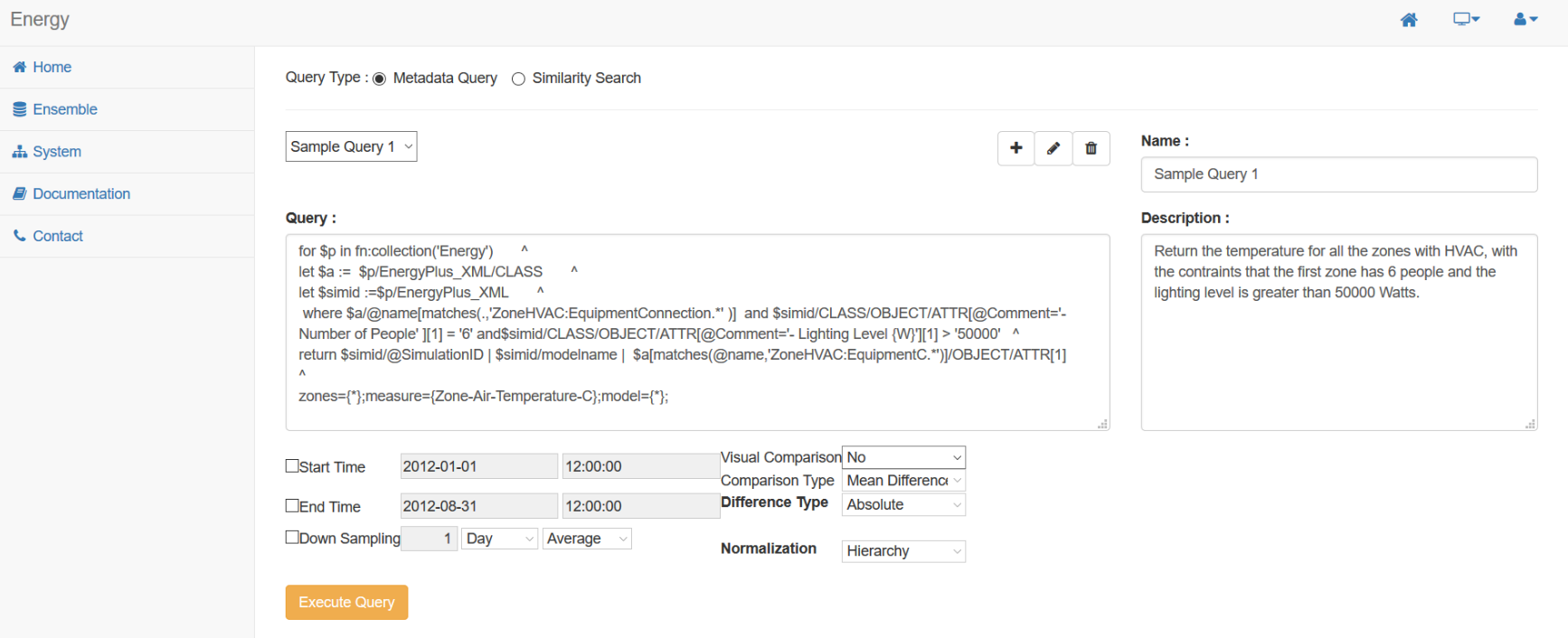
When conducting a metadata query, choose a saved query from the dropdown. Your query will be inserted into the query field, where final modifications can be made. Below, several additional filtering options are available to help refine the results. Once all settings have been finalized, click 'Execute Query' to perform the analysis. An example of this interface can be seen here:
When conducting a similarity search, the inputs are slightly different. Instead of choosing an existing query, you will need to supply two source files to use as a basis for comparison. The input formats are identical to the Data Management requirements for ensembles, specifically CSV format in the standard STEM format. Once supplied, the dropdowns can be used to select which data to search. Finally, click 'Search Similar Series' to perform the analysis.
Once your query is complete, the results will appear immediately underneath the query section. At first, it will appear as a simple hierarchical display, as seen here from the query over energy dataset above:
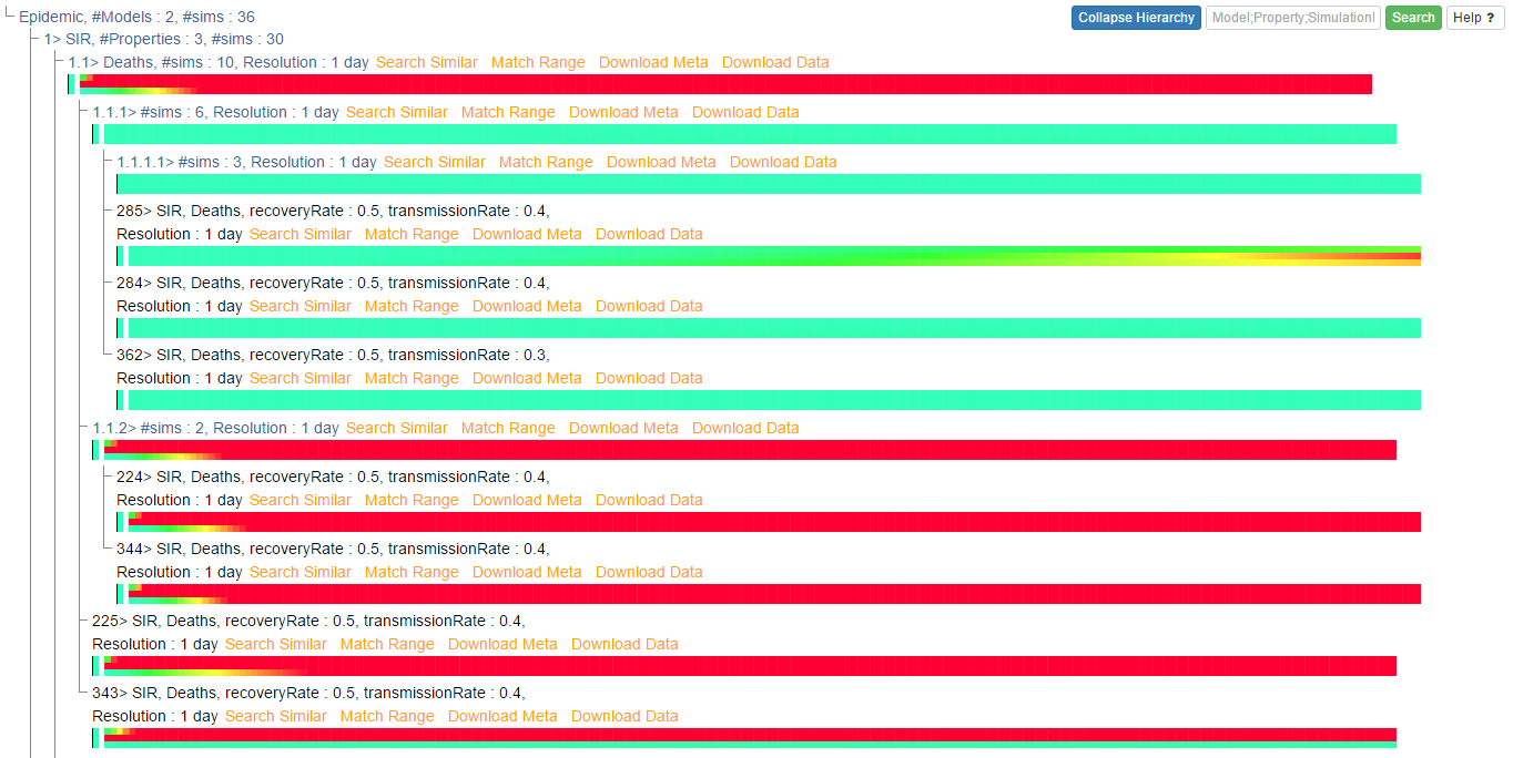
Alternatively, the hierarchical display of queries over epidemic dataset can be:
Click on any entry text in the hierarchy to expand that subtree. The number and depth of the subtrees will be dependent on the composition and complexity of the query. At any time, you may collapse the entire hierarchy by clicking the 'Collapse Hierarchy' button at the upper-right.
After the subtrees have been sufficiently expanded, result heatmaps will appear under their associated subquery headings. These heatmaps represent the time series data, with time on the X-axis and dimensions on the Y-axis:
Similar queries over epidemic dataset will generate data heatmaps like below:
For additional detail, any heatmap can be clicked to pop open a new window containing the Detailed View. This view allows users to refine the data using additional filters, provides access to more functiality such as downloading the time series or metadata, and labels the heatmap Y-axis with the relevant information.
This view should be used when additional information needs to be extracted from a specific region, or when users would like to drill down further into an analysis. An example can be seen here:
As query results become more complex, it may be desirable to find particular pieces of information within the results without searching for them manually. The 'Search' button at the upper-right of the results hierarchy can be used for this purpose.
Enter in the desired attribute to search for, followed by a ;, and then click the 'Search' button. This will filter the results to only display entries within the hierarchy that match the given pattern:


