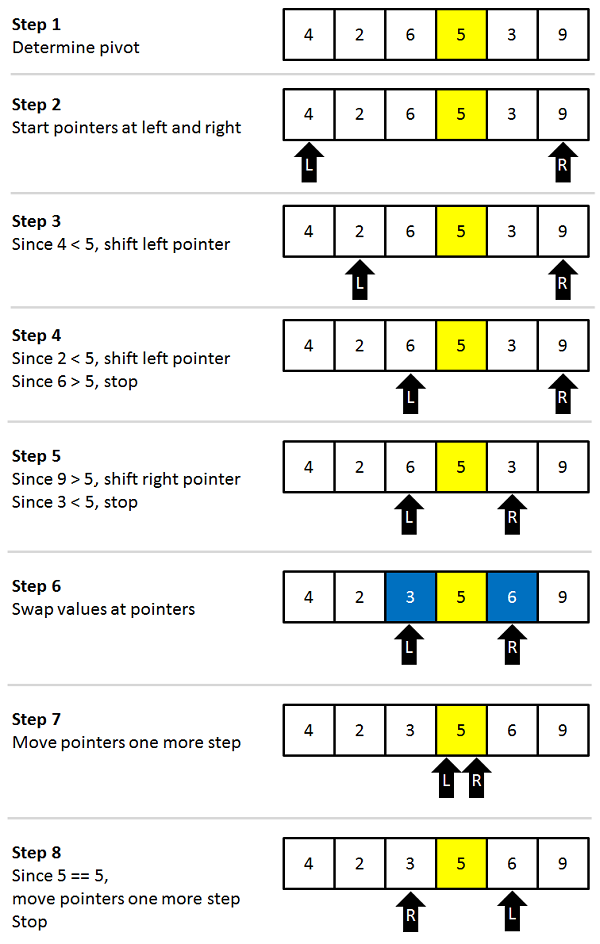
Quick_Sort

Quick Sort

QuickSort is one of the most efficient sorting algorithms and is based on the splitting of an array into smaller ones. The name comes from the fact that, quick sort is capable of sorting a list of data elements significantly faster than any of the common sorting algorithms. And like Merge sort, Quick sort also falls into the category of divide and conquer approach of problem-solving methodology.

Algorithm

1. Find a “pivot” item in the array. This item is the basis for comparison for a single round.
2. Start a pointer (the left pointer) at the first item in the array.
3. Start a pointer (the right pointer) at the last item in the array.
4. While the value at the left pointer in the array is less than the pivot value, move the left pointer to the right (add 1). Continue until the value at the left pointer is greater than or equal to the pivot value.
5. While the value at the right pointer in the array is greater than the pivot value, move the right pointer to the left (subtract 1). Continue until the value at the right pointer is less than or equal to the pivot value.
6. If the left pointer is less than or equal to the right pointer, then swap the values at these locations in the array.
7. Move the left pointer to the right by one and the right pointer to the left by one.
8. If the left pointer and right pointer don’t meet, go to step 1.

Pseudocode

The pseudocode for Quick Sort is as follows:

quicksort(A,p,r) {
    if (p < r) {
       q <- Partition(A,p,r)
       Quicksort(A,p,q)
       Quicksort(A,q+1,r)
    }
}

partition(A,p,r)
    x <- A[p]
    i <- p-1
    j <- r+1
    while (true) {
        repeat
            j <- j-1
        until (A[j] <= x)
        repeat
            i <- i+1
        until (A[i] >= x)
        if (i A[j]
        else 
            return(j)
    }
}

Example 1(Interactive)

Example 2(With explanation)

Below given is an array, which needs to be sorted. We will use the Quick Sort Algorithm to sort this array(this example chooses any element as pivot):

• After the above step, the first pivot is in its required place, similarly we sort the left and right halves of the array in a recursive manner.

Example 3(A different case)

Consider the following unsorted array, which needs to be sorted. We will consider the last element as pivot in this case.

[10, 80, 30, 90, 40, 50, 70]

Here are the steps:

• Pass 1:

  • Value of variables: i = -1, j = 0 | Test condition: arr[j] <= pivot (10 < 70 : True) | Actions: i++, swap(arr[i], arr[j]) | Array: [10, 80, 30, 90, 40, 50, 70]

• Pass 2:

  • Value of variables: i = 0, j = 1 | Test condition: arr[j] <= pivot (80 < 70 : False) | Actions: No Action | Array: [10, 80, 30, 90, 40, 50, 70]

• Pass 3:

  • Value of variables: i = 0, j = 2 | Test condition: arr[j] <= pivot (30 < 70 : True) | Actions: i++, swap(arr[i], arr[j]) | Array: [10, 30, 80, 90, 40, 50, 70]

• Pass 4:

  • Value of variables: i = 1, j = 3 | Test condition: arr[j] <= pivot (90 < 70 : False) | Actions: No Action | Array: [10, 30, 80, 90, 40, 50, 70]

• Pass 5:

  • Value of variables: i = 1, j = 4 | Test condition: arr[j] <= pivot (40 < 70: True) | Actions: i++, swap(arr[i], arr[j]) | Array: [10, 30, 40, 90, 80, 50, 70]

• Pass 6:

  • Value of variables: i = 2, j = 5 | Test condition: arr[j] <= pivot (50 < 70: True) | Actions: i++, swap(arr[i], arr[j]) | Array: [10, 30, 40, 50, 80, 90, 70]

• Before pass 7, j becomes 6, so we come out of the loop and now swap(arr[i+1], pivot) | Array: [10, 30, 40, 50, 70, 90, 80

• Now 70 is in its position, so we call quicksort function again on the left and right halves.

• Since the left part of 70 is already sorted, everytime the partition function is called, the pivot(i.e the last elements is already in its desired position)

• For the right half, after swapping 80 and 90, the pivot is brought to its desired position and now the entire array is sorted.

Complexity

The Time Complexity of Quick Sort is O(nLogn). In the worst case, it becomes O(n^2).

The Space Complexity of Quick Sort is O(Logn).