Intro
- The main hypothesis that motivates ADR is that training on a maximally diverse distribution over environments leads to transfer via emergent meta-learning.
- More concretely, if the model has some form of memory then it can learn to adjust its behavior during deployment to improve performance on the current environment.
- It is hypothesized that this happens if the training distribution is so large that the model cannot memorize a special purpose solution per environment as a result of its finite capacity.
- ADR is a first step in this direction of unbounded environmental complexity; it automates and gradially expands the randomization ranges that parameterize a distribution over environments.
Overview
- At its core ADR realizes a training curriculum that gradually expands a distribution over nvironments for which the model can perform well.
- The initial distribution over environments is concentrated on a single environment.
- The distribution over environments is sampled to obtain environments and evaluate model performance.
- ADR is independent of the algorithm used for model training - it only generates training data, so it can be used for both supervised and reinforcement learning.
Practical Matters
- The meat of the logic and implementation resides in the auto_dr/randomization folder.
- The Randomizer class wraps parallelized environments and adjusts their entropy depending on the performance of the agent.
- A fairly custom environment setup is required (such as this one for 2D-Navigation) which includes clear definitions for parameter bounds and values.
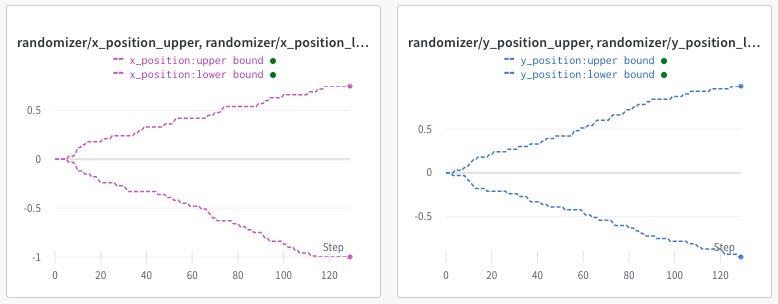
- In the 2D-Navigation environment where the agent's goal is to reach a specific point, the environment parameterization is progressively updated by widening the range of possible goal states (plotted below) as agent performance improves.
Parameter Bounds
Entropy & Ranges
Benefits of ADR
- Using a curriculum that gradually increases in difficulty as training progresses simplifies training, since the problem is solved on a single environment and additional environments are only added when some minimum performance is achieved.
- Acceptable performance is defined by performance thresholds, for policy training they are defined as the number of successes in an episode.
- During evaluations, we compute the percentage of samples that achieve acceptable performance - if the resulting percentage is above the upper threshold or the lower threshold then the distribution is adjusted accordingly.
- It removes the need to manually tune the randomizations - this is critical, since as more randomization parameters are incorporated, manual adjustment becomes increasingly difficult and non-intuitive.
Algorithm
- Each environment
$e_\lambda$ is parameterized by$\lambda \in \mathbb{R}^d$ where d is the number of parameters we can randomize in simulation. - In domain randomization, the parameter
$\lambda$ comes from a fixed distribution$P\phi$ parameterized by$\phi \in \mathbb{R}^{d'}$ . - In ADR, the parameterization
$\phi$ of the distribution of the environment parameters$\lambda$ is changing dynamically with training progress. - To quantify the ADR expansion, ADR entropy is defined as (a higher ADR entropy is associated with a broader distribution),
$$H(P_\phi) = -\frac{1}{d} \int P_{\phi}(\lambda) \space log P_{\phi}(\lambda)d\lambda$$ - In ADR, a factorized distribution parameterized by d' = 2d parameters is used.
- For the i-th ADR parameter
$\lambda_i$ ,$i = 1, 2, ..., d$ the pair$(\phi_i^L, \phi_i^H)$ is used to describe a uniform distribution for sampling$\lambda_i$ such that$\lambda_i \sim U(\phi_i^L, \phi_i^H)$ . - The boundary values are inclusive so that the overall distribution is given by,
- The ADR entropy is measured as
- At each iteration, the ADR algorithm randomly selects a parameter of the environment to fix to a boundary value
$\phi_i^L$ or$\phi_i^H$ while the other parameters are sampled as per$P_{\phi}$ - this is referred to as boundary sampling. - Evaluation of thresholds,
- Model performance for the sampled environment is then evaluated and appended to the buffer associated with the selected boundary.
- Once enough performance data is collected it is averaged and compared to the thresholds.
- If average model performance is better than the high threshold, the parameter for the chosen dimension is increased.
- On the other hand, the parameter is decreased if the average model performance is worse than the low threshold.
Reference
- Solving Rubik's Cube with a Robot Hand https://arxiv.org/abs/1910.07113

