####1. Enabling I2C
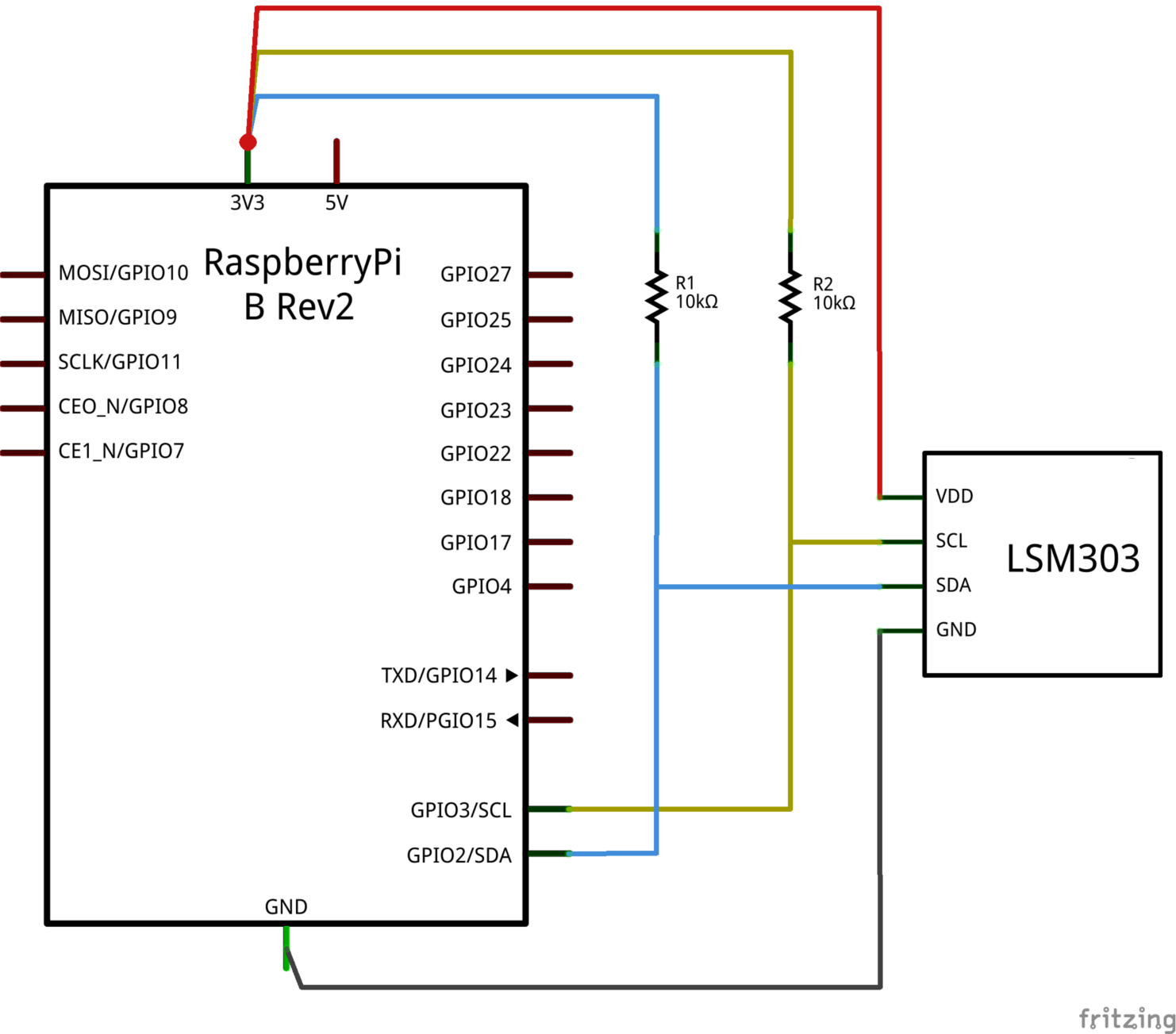
The Raspberry Pi has a single I2C channel on pins 3 (SDA) and 5 (SCL). By default the I2C channel is disabled. To enable it, follow steps 1-4 in the instructions on this page with only one item to note. Once the files have been edited and it is time to run the i2cdetect tool, the identifying number needs to be correct. The instructions say to use 0, but it could be it needs to be 1. To verify run the following commands in the terminal
$ cd /dev
$ ls | grep i2c
This will list the I2C interfaces on the Raspberry Pi. The number at the end is the argument to pass to i2cdetect. For example, if running the command returned
i2c-1
the i2cdetect tool should be run with
$ i2cdetect -y 1
The following diagram shows the schematic used for this example
####2. Writing the Code
The code provided is written in Python and works with a LSM303DLHC 3D compass and accelerometer. The code utilizing it is by no means meant to be a complete solution for this device. It simply provides an example to demonstrate how to program the I2C interface. It will only be making use of the accelerometer capabilities. The magnetometer can be utilized in a similar fashion. The file lsm303.py contains the complete source code for this example. It contains some code for the magnetometer, but it doesn't really do anything useful with it. It is there just to provide a bit of a starting point.
#####2.1 Importing smbus
The smbus package contains the classes used for I2C communication. At the top of the Python script add the line
import smbus
#####2.2 Creating the SMBus Object
The communication with the I2C bus happens using the SMBus object. Its constructor requires an index identifying which I2C bus to use. The following line of code will instantiate a SMBus object that will communicate over bus 1.
bus = smbus.SMBus(1)
#####2.3 About the SMBus Object
For this example we will be using only two functions from the SMBus class: write_byte_data() and read_byte_data(). Documentation for these and other functions can be found here. The function signature for write_byte_data() is
write_byte_data(addr, cmd, val)
where addr is the address of the I2C component, cmd is the command to be run or the register to write to, and val is the value to be written. The function signature for read_byte_data() is
read_byte_data(addr, cmd)
where addr is the address of the I2C component and cmd is the command to be run or the register to be read.
#####2.4 Initializing the Accelerometer
After creating the SMBus object, we can use it to configure our accelerometer. The following code snippet configures the accelerometer to update acceleration data at a rate of 50 Hz and enables all three axes. It also sets our linear acceleration full scale to +/- 4G.
LIN_ACCEL_ADDR = 0x19
LIN_ACCEL_REG_CTRL_REG1_A = 0x20
LIN_ACCEL_REG_CTRL_REG4_A = 0x23

bus.write_byte_data(LIN_ACCEL_ADDR, LIN_ACCEL_REG_CTRL_REG1_A, 0x47)
bus.write_byte_data(LIN_ACCEL_ADDR, LIN_ACCEL_REG_CTRL_REG4_A, 0x90)
#####2.5 Reading the Accelerometer
Once the accelerometer has been initialized, the SMBus object can be used to read data from its registers. The following code snippet is a helper function that reads data from a given register.
def read_accel_reg(register):
    return bus.read_byte_data(LIN_ACCEL_ADDR, register)
The next code snippet uses this function to read the raw x-acceleration data and turns it into a signed integer where 0 acceleration corresponds to a 0 value.
LIN_ACCEL_REG_OUT_X_L_A = 0x28
LIN_ACCEL_REG_OUT_X_H_A = 0x29

def read_x_accel():
    lo = read_accel_reg(LIN_ACCEL_REG_OUT_X_L_A)
    hi = read_accel_reg(LIN_ACCEL_REG_OUT_X_H_A)
    total = (hi << 8) + lo
    total = convert_twos_complement(total)
    return total
After initially constructing the value total, it is used by the code as an unsigned integer value. It needs to be turned into a signed integer centered at 0. This is done by the convert_twos_complement() function. Its definition can be found in the source code.
#####2.6 Making Acceleration Values Useful
The read_x_accel() function can be modified to convert the acceleration value into an acceleration value in meters/second^2. The following code snippet modifies the previous read_x_accel() function to convert to m/s^2
G_RESOLUTION = 32768 / 4
G_TO_M_S2 = 9.80665

def read_x_accel():
    lo = read_accel_reg(LIN_ACCEL_REG_OUT_X_L_A)
    hi = read_accel_reg(LIN_ACCEL_REG_OUT_X_H_A)
    total = (hi << 8) + lo
    total = convert_twos_complement(total)

    return (float(total) / float(G_RESOLUTION)) * G_TO_M_S2
Here G_RESOLUTION is a constant that specifies an integer value per g. In this case, if the accelerometer gives a value of 8192 it corresponds to 1 g, 16384 corresponds to 2 g, etc. Likewise, -8192 corresponds to -1 g, -16384 corresponds to -2 g, etc.
#####2.7 Using it in ROS
Now that the acceleration values are available they can start being used in ROS. The following code snippet hows how this can be done.
import rospy
from sensor_msgs.msg import Imu

G_RESOLUTION = 32768 / 4
G_TO_M_S2 = 9.80665

LIN_ACCEL_ADDR = 0x19
LIN_ACCEL_REG_CTRL_REG1_A = 0x20
LIN_ACCEL_REG_CTRL_REG4_A = 0x23
LIN_ACCEL_REG_OUT_X_L_A = 0x28
LIN_ACCEL_REG_OUT_X_H_A = 0x29
LIN_ACCEL_REG_OUT_Y_L_A = 0x2A
LIN_ACCEL_REG_OUT_Y_H_A = 0x2B
LIN_ACCEL_REG_OUT_Z_L_A = 0x2C
LIN_ACCEL_REG_OUT_Z_H_A = 0x2D

bus = smbus.SMBus(1)

imu_pub = rospy.Publisher("lin_accel", Imu, queue_size=10)

def run():
    # Initialize/configure the accelerometer
    bus.write_byte_data(LIN_ACCEL_ADDR, LIN_ACCEL_REG_CTRL_REG1_A, 0x47)
    bus.write_byte_data(LIN_ACCEL_ADDR, LIN_ACCEL_REG_CTRL_REG4_A, 0x90)

    # Get the node up and running so it can publish acceleration data.
    rospy.init_node("lsm303", anonymous=True)
    rospy.Timer(rospy.Duration(0.1), timer_callback)
    rospy.spin()

def timer_callback(event):
    global imu_pub

    # Read our acceleration values.
    x_accel = get_x_accel()
    y_accel = get_y_accel()
    z_accel = get_z_accel()

    # Stuff the acceleration values into an Imu message and send it out.
    imu_msg = Imu()
    imu_msg.header.stamp = rospy.Time.now()
    imu_msg.linear_acceleration.x = x_accel
    imu_msg.linear_acceleration.y = y_accel
    imu_msg.linear_acceleration.z = z_accel
    imu_pub.publish(imu_msg)
Now that the code is ready, the node can be run in order to publish data. Make sure roscore is running in a separate terminal. Also ensure the command
$ source devel/setup.bash
has been run from the root of the current workspace. Then run the command
$ rosrun rpi_examples_indigo lsm303.py
to start publishing acceleration data.
#####2.8 Publishing the tf Data
Now that the acceleration data is being published it can be viewed in rviz on another machine. This can be done by subscribing to the /lin_accel topic, updating the velocity and position of the Raspberry Pi, and publishing new tf data. The source code for this example can be found in pi_position.py. Information on tf can be found in this documentation and these tutorials.
First a subscriber needs to be created.
rospy.Subscriber("/lin_accel", Imu, received_callback)
Next a tf.TransformBroadcaster needs to be created. Once these are finished the acceleration data can be used to generate a new position for the Raspberry Pi.
def received_callback(data):
    current_time_s = rospy.get_time()
    if prev_time_s != 0.0:
        delta_t = current_time_s - prev_time_s

        x_pos += v_x * delta_t
        y_pos += v_y * delta_t
        z_pos += v_z * delta_t

        v_x += data.linear_acceleration.x * delta_t
        v_y += data.linear_acceleration.y * delta_t
        v_z += data.linear_acceleration.z * delta_t

        br.sendTransform((x_pos, y_pos, z_pos),
            tf.transformations.quaternion_from_euler(0.0, 0.0, 0.0),
            rospy.Time.now(),
            "base_link",
            "world")

    prev_time_s = current_time_s
The call to sendTransform() will transmit the tf data to be used by the rest of ROS, and specifically rviz. The function received_callback() will be called any time linear acceleration data is received.
As an additional note, the full code contains offsets that can be applied to the x-, y-, and z-acceleration values to try to get them closer to 0.0 when at rest. These values naively assume that the accelerometer never rotates or changes orientation. If this happens, gravity causes the values to shift, which will mess up all of the calculations. Compensating for gravity requires knowing the orientation (roll, pitch, yaw) of the accelerometer, which is not available in this code.
#####2.9 Plot the acceleration data
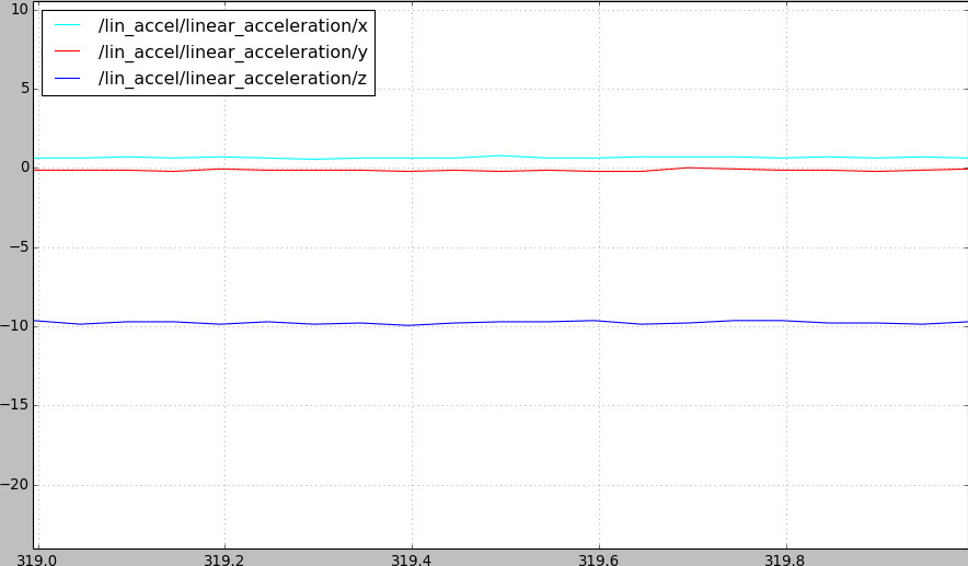
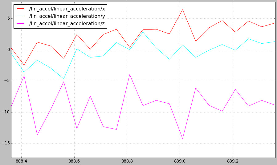
Now use rqt_plot to plot the message of the acceleration data. We could get something similar to the following
This will need to be done on a remote machine. Before attempting to do so, ensure the network between the Raspberry Pi and a remote machine has been setup according to the instructions on the home page of this documentation. Once the everything is setup, run
$ rqt_plot
from a terminal to launch the program. The values coming from the Raspberry Pi can now be plotted in real-time.
#####2.10 Preparing to View in rviz
The data is waiting to be viewed in rviz. Before doing that, the network needs to be setup. Make sure the Raspberry Pi and remote machine have their network settings set as mentioned in the home page of this documentation so that the remote machine can received acceleration data from the Raspberry Pi.
#####2.11 Viewing it in rviz
Now that the tf data is being published, the movement of the Raspberry Pi can be viewed in rviz once a URDF file has been created. For the purposes of this example a simple URDF will suffice, such as the one shown in the following snippet (this snippet shows the contents of accels.urdf).
<?xml version="1.0"?>
<robot name="pi_accels">
  <link name="base_link">
    <visual>
      <geometry>
    <box size="0.6 0.2 0.1"/>
      </geometry>
    </visual>
  </link>
</robot>
This file defines a single box link, which is sufficient for showing the Raspberry Pi's position in space. For more information regarding URDF files see these tutorials and this information on the XML tags.
Now it is time to launch the node as well as rviz to view the URDF file. To help with loading the URDF file and launching rviz, the file pi_in_rviz.launch has been created. It launches the pi_position.py file and also launches the display.launch file from the urdf_tutorial. This code snippet displays the contents of pi_in_rviz.launch
<?xml version="1.0"?>
<launch>
  <node name="pi_position" pkg="rpi_examples_indigo" type="pi_position.py">
      <param name="_x_offset" value="-0.641"/>
      <param name="_y_offset" value="0.14"/>
      <param name="_z_offset" value="9.74"/>
      <param name="_print_debug" value="False"/>
  </node>

  <include file="$(find urdf_tutorial)/launch/display.launch">
      <arg name="model" value="accels.urdf"/>
  </include>
</launch>
The display.launch file from urdf_tutorial loads a URDF file and launches rviz. The urdf file is specified by the entry
<arg name="model" value="accels.urdf"/>
Notice that there are several offset parameters with values set. These correspond to the acceleration offset values to try to zero the values as much as possible. These should be tuned for each accelerometer. The _print_debug parameter can be used to print accelerations and velocities to the console so that the offsets can be tuned more easily.
To launch everything run the command
roslaunch rpi_examples_indigo pi_in_rviz.launch
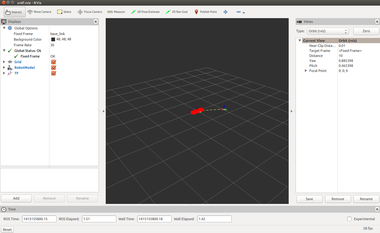
and move the Raspberry Pi around to see it move in rviz. The following image demonstrates how it might look.
Notice in the left-hand column of the image that the Fixed Frame entry is set to base_link. This means the base_link will be the fixed point while the world frame moves relative to it. To see the box move instead, change Fixed Frame to world.


