-
Notifications
You must be signed in to change notification settings - Fork 37
/
README.Rmd
130 lines (92 loc) · 6.18 KB
/
README.Rmd
1
2
3
4
5
6
7
8
9
10
11
12
13
14
15
16
17
18
19
20
21
22
23
24
25
26
27
28
29
30
31
32
33
34
35
36
37
38
39
40
41
42
43
44
45
46
47
48
49
50
51
52
53
54
55
56
57
58
59
60
61
62
63
64
65
66
67
68
69
70
71
72
73
74
75
76
77
78
79
80
81
82
83
84
85
86
87
88
89
90
91
92
93
94
95
96
97
98
99
100
101
102
103
104
105
106
107
108
109
110
111
112
113
114
115
116
117
118
119
120
121
122
123
124
125
126
127
128
---
output:
- md_document
---
# esri2sf
Scraping Geographic Features from ArcGIS Server
Still many geographic data is delivered through ESRI's ArcGIS Server.
It is not easy to utilize the geographic data in the GIS servers from data analysis platform like R or Pandas.
This package enables users to scrape vector data in ArcGIS Server from R through the server's REST API.
It download geographic features from ArcGIS Server and saves it as [Simple Features](https://cran.r-project.org/web/packages/sf/vignettes/sf1.html).
## How it works
This program sends a request to an ArcGIS Server and gets json responses containing coordinates of geometries
of which format is not the same as geojson. So it converts the json into simple feature geometries from the response.
Then it combines attribute data to the geometries to create sf dataframe.
Often ArcGIS servers limits the maximum number of rows in the result set. So this program
creates 500 features per request and automatically re-send requests until it gets all features in the dataset.
## Install
Use [remotes](https://cran.r-project.org/web/packages/remotes/index.html) to install this package. This package has dependencies on dplyr, sf, httr, jsonlite, rstudioapi, DBI, RSQLite, crayon and rmarkdown, knitr, and pbapply are suggested.
```R
library(remotes)
install_github("yonghah/esri2sf")
```
## How to use
What you need is the URL of REST service you want. You can get the URL by viewing the URL widget on the service's webpage (see image below),
by asking a GIS admin, or looking at the javascript code of a webpage where it creates a feature layer.

### Point data
```{R points}
library("esri2sf")
url <- "https://services.arcgis.com/V6ZHFr6zdgNZuVG0/arcgis/rest/services/Landscape_Trees/FeatureServer/0"
df <- esri2sf(url)
plot(df)
```
<!--  -->
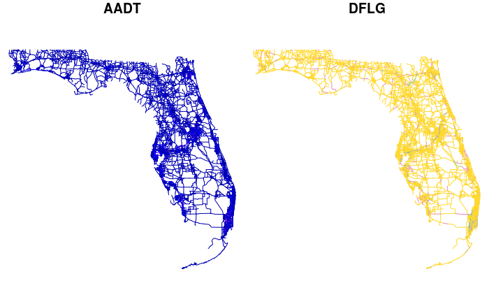
### Polyline data
You can filter output fields. This may take a minute since it gets 18000 polylines.
```{R polyline}
url <- "https://services.arcgis.com/V6ZHFr6zdgNZuVG0/arcgis/rest/services/Florida_Annual_Average_Daily_Traffic/FeatureServer/0"
df <- esri2sf(url, outFields=c("AADT", "DFLG"))
plot(df)
```
<!--  -->
### Polygon data
You can filter rows as well by giving a `where` condition.
```{R polygon}
url <- "https://sampleserver1.arcgisonline.com/ArcGIS/rest/services/Demographics/ESRI_Census_USA/MapServer/3"
df <- esri2sf(url,
where = "STATE_NAME = 'Michigan'",
outFields = c("POP2000", "pop2007", "POP00_SQMI", "POP07_SQMI"))
plot(df)
```
<!--  -->
### Tabular data
You can download non-spatial tables of the 'Table' layer type using `esri2df()`.
```{r tables}
df <- esri2df('https://sampleserver1.arcgisonline.com/ArcGIS/rest/services/WaterTemplate/WaterDistributionInventoryReport/MapServer/5', objectIds = paste(1:50, collapse = ","))
df
```
### `crs` parameter example
When specifying the CRS parameter, any transformation that happens will be done within ESRI's REST API. Caution should be taken when specifying an output `crs` that requires a datum transformation as ESRI will automatically apply a default transformation (with no feedback as to which one) which could end up adding small unexpected errors into your data. By default, `esri2sf()` will transform any datasource to WGS 1984 (EPSG:4326), but it may be safer to set `crs = NULL` which will return the data in the same CRS as it is being hosted as in the Feature/Map Service. That way you can control any transformation manually in a known, reproducible manner.
```{r}
url <- "https://sampleserver1.arcgisonline.com/ArcGIS/rest/services/Demographics/ESRI_Census_USA/MapServer/3"
where <- "STATE_NAME = 'Michigan'"
outFields <- c("POP2000", "pop2007", "POP00_SQMI", "POP07_SQMI")
#default crs = 4326
esri2sf(url, where = where, outFields = outFields)
#No transformation (recommended)
esri2sf(url, where = where, outFields = outFields, crs = NULL)
```
Also since the addition of the `WKT1_ESRI` output from sf::st_crs() in sf version 1.0-1, you can enter common CRS format (any that sf::st_crs() can handle) into the `crs` parameters and it will be able to convert to the ESRI formatted WKT needed for the outSR field in the REST query. Below are examples of the variety of input types that you can use with the `crs` parameters. All examples are just different formulations of the ESRI:102690 CRS.
```{r}
#ESRI Authority Code
df1 <- esri2sf(url, where = where, outFields = outFields, crs = "ESRI:102690")
#PROJ string
df2 <- esri2sf(url, where = where, outFields = outFields, crs = "+proj=lcc +lat_1=42.1 +lat_2=43.66666666666666 +lat_0=41.5 +lon_0=-84.36666666666666 +x_0=4000000 +y_0=0 +datum=NAD83 +units=us-ft +no_defs")
#OGC WKT
df3 <- esri2sf(url, where = where, outFields = outFields, crs = 'PROJCS["NAD_1983_StatePlane_Michigan_South_FIPS_2113_Feet",GEOGCS["GCS_North_American_1983",DATUM["North_American_Datum_1983",SPHEROID["GRS_1980",6378137,298.257222101]],PRIMEM["Greenwich",0],UNIT["Degree",0.017453292519943295]],PROJECTION["Lambert_Conformal_Conic_2SP"],PARAMETER["False_Easting",13123333.33333333],PARAMETER["False_Northing",0],PARAMETER["Central_Meridian",-84.36666666666666],PARAMETER["Standard_Parallel_1",42.1],PARAMETER["Standard_Parallel_2",43.66666666666666],PARAMETER["Latitude_Of_Origin",41.5],UNIT["Foot_US",0.30480060960121924],AUTHORITY["EPSG","102690"]]')
```
Their similarity on the output CRS can be proven by the following function that calculates the mean difference in X-Y coordinates at each point. All are very close to 0.
```{r}
coord_diff <- function(df1, df2) {
suppressWarnings({
c(
"x" = mean(sf::st_coordinates(sf::st_cast(df1, "POINT"))[,1] - sf::st_coordinates(sf::st_cast(df2, "POINT"))[,1]),
"y" = mean(sf::st_coordinates(sf::st_cast(df1, "POINT"))[,2] - sf::st_coordinates(sf::st_cast(df2, "POINT"))[,2])
)
})
}
coord_diff(df1, df2)
coord_diff(df1, df3)
coord_diff(df2, df3)
```