BERT: Inference Optimization with TensorRT

BERT (Bidirectional Encoder Representations from Transformers) is a deep learning model introduced by Google AI Language team in 2018, capable of handling various NLP tasks. Previously, each NLP task typically required a specific model to solve. However, BERT's emergence changed this landscape. At the time, it could handle over 11 common NLP tasks and outperformed previous models in performance. Before the advent of large language models, BERT-based models and their variants were the universal solution in the NLP field.

We will elaborate on BERT and model inference optimization points in the following 5 sections:

1. BERT's Applications and How It Works

1.1 BERT's Applications

BERT, as an advanced language processing model, plays a crucial role in various language tasks:

• Sentiment Analysis：BERT can analyze texts like movie reviews to determine whether the sentiment is positive or negative.
• Question Answering Systems：It can provide capabilities for chatbots, enabling them to understand better and answer user questions.
• Text Prediction：When writing texts like emails, BERT can predict words or phrases the user might input next, such as Gmail's smart compose feature.
• Text Generation：BERT can also generate an article on a specific topic based on a few given sentences.
• Text Summarization：It can quickly extract key information from long texts, like legal contracts, to generate summaries.
• Disambiguation：BERT can accurately understand and distinguish ambiguous words based on context, for example, "Bank" can refer to a financial institution or a riverbank.

These are just a part of BERT's capabilities. In fact, BERT and other NLP technologies have permeated many aspects of our daily lives:

• Translation Services: Tools like Google Translate use NLP technology to provide accurate language translation.
• Voice Assistants: Voice assistants like Alexa and Siri rely on NLP to understand and respond to users' voice commands.
• Chatbots: Online customer service and chatbots use NLP to parse users' questions and provide useful answers.
• Search Engines: Google Search uses NLP technology to understand the intent of search queries and provide relevant results.
• Voice Navigation: GPS and navigation applications use voice control features, allowing users to operate through voice commands.

As shown in the image above, Google Translate, since 2020, BERT has been helping Google better display results for almost all (English) searches.

1.2 How BERT Works

BERT's working principle is mainly based on the following key concepts:

• Transformer Model: The Transformer is a deep learning architecture, its core is the attention mechanism, which allows the model to process sequence data and capture long-distance dependencies in the sequence.
• Bidirectional Training: Traditional language models only consider one direction of the text during training, either from left to right or right to left. BERT is bidirectional, considering the entire text at once, allowing BERT to understand the context of words.
• Pre-training and Fine-tuning: BERT is first pre-trained on a large amount of text data, then fine-tuned on specific tasks. The goal of the pre-training phase is to understand the grammar and semantics of language (through two tasks: masked language model and next sentence prediction). The fine-tuning phase is to make the model understand specific tasks (such as sentiment analysis or question answering).
• Word Embedding: BERT uses WordPiece embedding, which is a subword embedding method. This means BERT can handle out-of-vocabulary words because it can break words down into known subwords.

In practical use, the BERT model receives a string of tokens (usually words or subwords) as input, then outputs the embeddings of these tokens, which are obtained by considering the context (i.e., other tokens in the input sequence). These embeddings can then be used for various downstream tasks such as text classification, named entity recognition, or question answering.

We are more focused on BERT's inference process, so we won't elaborate on training and fine-tuning here. The most important aspects are the Transformer structure and the word embedding method, which we will elaborate on in detail later. Simply put, the text input is converted to a tensor through the word embedding layer, then executes the Encoder layers of the Transformer structure, goes through multiple layers, and obtains an output tensor. Specific post-processing is performed for specific tasks. For example, if it's a classification task, it goes through a linear layer and softmax layer and other classification modules to return the probability of each category; if it's a translation service, it returns the text information corresponding to the tensor.

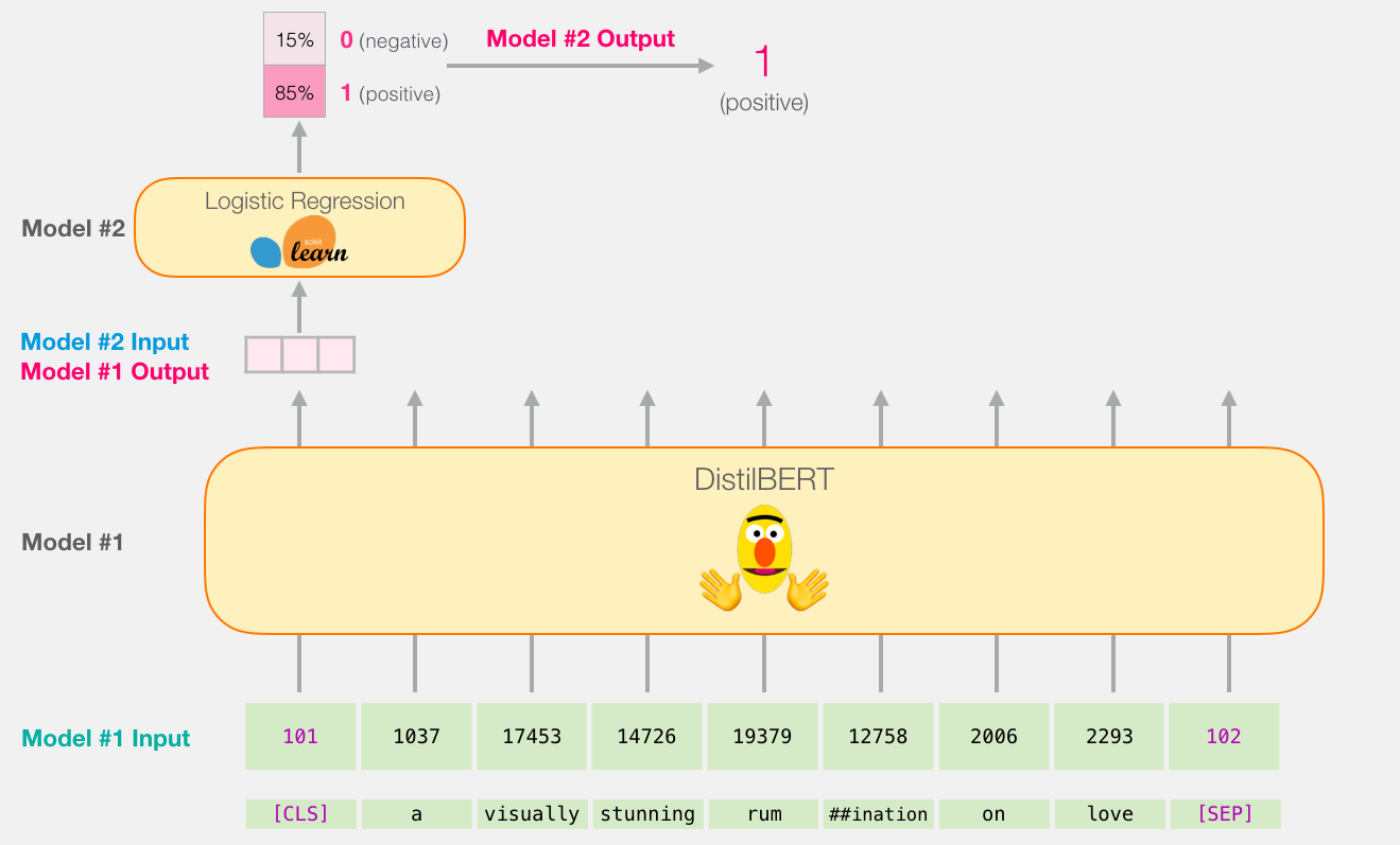
The above image shows the workflow of a sentiment classification task for BERT. The input "a visually stunning rumination on love" goes through the Tokenize layer, Embedding layer, and Encoder layer to get BERT's output, then goes through a Logistic Regression layer to get the probabilities of "positive" and "negative", and finally gets the sentiment classification result as "positive".

2. BERT Model Structure and Size

The BERT model is primarily composed of the Tokenizer layer, Embedding layer, and Encoder layers. The Encoder layer includes the Self-Attention layer, LayerNorm, Feed Forward layer, and Residual Connection & Normalization layer.

2.1 Tokenizer Layer

The Tokenizer layer is responsible for converting raw text into a format that the BERT model can understand and process. This conversion process involves the following steps:

• Tokenization: The raw text is split into words or subword units. BERT uses the WordPiece algorithm, which can break down unknown or rare words into smaller, known subwords.
• Adding Special Tokens: Special tokens such as [CLS] and [SEP] are added to mark the start and end of sentences. The [CLS] token is used for classification tasks, while the [SEP] token is used to separate paired sentences.
• Token to ID Conversion: Each token is converted to its corresponding ID in the vocabulary. The BERT vocabulary is fixed, with each word or subword having a unique index.
• Padding and Truncation: To process multiple sentences in batches, the BERT Tokenizer pads (or truncates) all sentences to the same length.
• Creating Attention Masks: An attention mask is created to indicate which positions are actual words and which are padding. This allows the model to ignore the padded parts during processing.

Input text

text = "Here is some text to encode"
# Process text using the tokenizer and return a tensor
encoded_input = tokenizer(text, return_tensors='pt')

In this example, encoded_input will be a dictionary containing the transformed input data, such as input_ids and attention_mask, which can be directly used by the BERT model.

2.2 Embedding Layer

In BERT, the Embedding layer, which is the first layer of the model, is responsible for converting input tokens into fixed-dimensional vectors. These vectors are numerical representations that the model can understand and process, encoding both the semantic information of words and their meanings in specific contexts.

The BERT embedding layer includes the following components:

• Token Embeddings: These are the basic embeddings that convert words or subword tokens into vectors. Each token is mapped to a point in a high-dimensional space (768 dimensions in the base BERT model).
• Segment Embeddings: BERT can process pairs of sentences (e.g., questions and answers in a QA task). Segment embeddings are used to distinguish between the two sentences, with each sentence being assigned a different segment embedding.
• Positional Embeddings: Since BERT uses a Transformer architecture, which doesn’t naturally handle sequential data like RNNs, positional embeddings are introduced to encode the position of each token in the sentence.

These three types of embeddings are added element-wise to produce a composite embedding, which encodes the token’s semantic information, its position in the sentence, and which sentence it belongs to (in the case of paired sentences). This composite embedding is then passed to the subsequent layers of BERT for further processing.

Here’s how it’s implemented in PyTorch:

# Initialization
self.token_embeddings = nn.Embedding(vocab_size, hidden_size)
self.segment_embeddings = nn.Embedding(type_vocab_size, hidden_size)
self.position_embeddings = nn.Embedding(max_position_embeddings, hidden_size)
# Usage
# Result of tokenization
seq_length = input_ids.size(1)
position_ids = torch.arange(seq_length, dtype=torch.long, device=input_ids.device)
position_ids = position_ids.unsqueeze(0).expand_as(input_ids)
# Get token embeddings from token ids
token_embeds = self.token_embeddings(input_ids)
# Get segment embeddings from segment ids
segment_embeds = self.segment_embeddings(segment_ids)
# Get position embeddings from position ids
position_embeds = self.position_embeddings(position_ids)

Internally, nn.Embedding contains a parameter matrix of size (num_embeddings, embedding_dim), which serves as the embedding matrix. When indices are passed in, PyTorch uses these indices as row numbers to retrieve the corresponding embedding vectors from the matrix. This process is highly efficient, especially on GPUs.

2.3 Encoder Layer

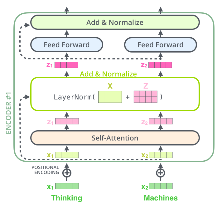
The Encoder and Decoder are two key components of the Transformer architecture, but BERT uses only the Encoder. BERT is composed of multiple stacked Encoder layers. The diagram below shows the structure of an Encoder, including the Attention layer, LayerNorm layer, Feed Forward layer, and Residual Connection & Normalization layer.

2.3.1 Self-Attention Layer

Self-attention can be understood as the process where words within a sentence pay attention to the influence of other words in the same sentence. In other words, it determines which words in the sentence should focus on which other words.

The core components of self-attention are the Query, Key, and Value vectors.

• Query (Q): This can be viewed as the element seeking information. For each word in the input sequence, a query vector is computed, representing what the word wants to focus on in the sequence.
• Key (K): Keys act like signposts, helping to identify and locate important elements in the sequence. Like the query, a key vector is computed for each word.
• Value (V): Values carry the information. Again, a value vector is computed for each word, containing the content that should be considered when determining the importance of words in the sequence.

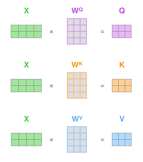
1. Computing Query, Key, and Value: For each word in the input sequence, query (Q), key (K), and value (V) vectors are computed. These vectors are the basis for the self-attention mechanism. Corresponding to these three vectors, there are three Linear layers. The input is multiplied by the weights of these three Linear layers to obtain the Q, K, and V vectors, as shown by the model weights $W^Q$, $W^K$, $W^V$ in the diagram below.

   

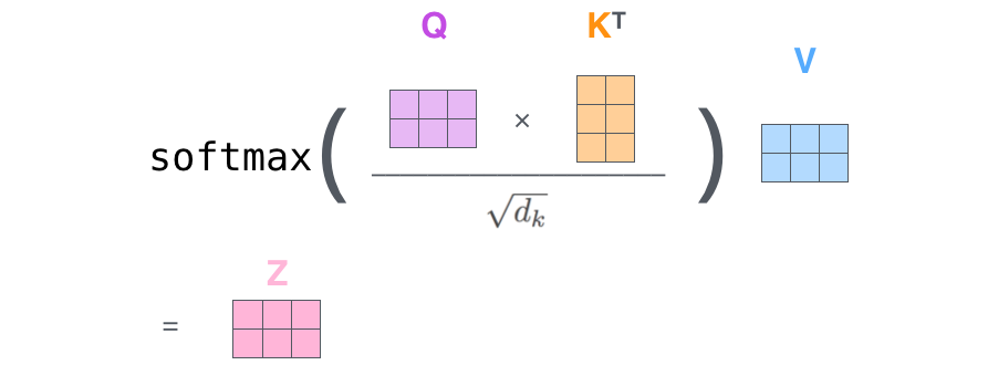
2. Computing Attention: For each word pair in the sequence, attention scores are calculated. The attention score between a query and key quantifies their relevance. The attention scores are computed by multiplying the Q vector and the transpose of the K vector, dividing by a parameter, and then applying a softmax function, followed by multiplying by the V vector. $$ Y = \text{softmax}\left(\frac{QK^T}{\sqrt{d_k}}\right)V $$

   

   Here, $QK^T$ is the dot product of two matrices; $d_k$ is the dimension of the Key, which generally matches the dimensions of Query and Value; $\text{softmax}$ is applied along the last dimension, row-wise.

   By this point, you may have a basic understanding of how the attention mechanism is expressed mathematically, but still be unsure why this process is effective. Let's use a simple example to better understand the role of attention. Consider the input sequence I met my teacher in the library yesterday. The word I might focus on yesterday to capture the time information; library might focus on my teacher to understand the relationship between location and person; met might focus on I and my teacher to understand who is acting and to whom.

   In the above input sequence, there are complex relationships between different components. Self-attention is used to extract these complex relationships.

3. Multi-Head Attention: This is an extension of self-attention, expanding the model's ability to focus on different parts of the sequence. Multi-head attention provides the attention layer with multiple "representation subspaces," allowing for richer levels of attention. With multi-head attention, there are multiple sets of Q, K, V weight matrices, leading to multiple results like those in steps 1 and 2. These results are then concatenated into a longer vector, and a fully connected network (matrix multiplication) is applied to produce a shorter output vector.

   

We can also understand the role of multi-head attention more intuitively. In explaining self-attention, we used an example of students in a classroom learning from each other. In that example, the students took only one comprehensive test to assess their Query, Key, and Value, but relying on just one test might lead to errors because some students might not perform well. The best approach would be to design multiple comprehensive tests to assess the students’ Query, Key, and Value as accurately as possible. This is essentially the role of multi-head self-attention.

Here’s how it’s implemented in PyTorch:

class MultiHeadAttention(nn.Module):
    def __init__(self):
        super(MultiHeadAttention, self).__init__()
        self.W_Q = nn.Linear(d_model, d_k * n_heads, bias=False)
        self.W_K = nn.Linear(d_model, d_k * n_heads, bias=False)
        self.W_V = nn.Linear(d_model, d_v * n_heads, bias=False)
        self.fc = nn.Linear(n_heads * d_v, d_model, bias=False)

    def forward(self, Q, K, V, attn_mask):
        '''
        Q, K, V: [batch, seq_len, d_model]
        attn_mask: [batch, seq_len, seq_len]
        '''
        batch = Q.size(0)
        '''
        split Q, K, V to per head formula: [batch, seq_len, n_heads, d_k]
        Convenient for matrix multiply opearation later
        q, k, v: [batch, n_heads, seq_len, d_k / d_v]
        '''
        per_Q = self.W_Q(Q).view(batch, -1, n_heads, d_k).transpose(1, 2)
        per_K = self.W_K(K).view(batch, -1, n_heads, d_k).transpose(1, 2)
        per_V = self.W_V(V).view(batch, -1, n_heads, d_v).transpose(1, 2)

        attn_mask = attn_mask.unsqueeze(1).repeat(1, n_heads, 1, 1)
        # context: [batch, n_heads, seq_len, d_v]
        context = ScaledDotProductAttention()(per_Q, per_K, per_V, attn_mask)
        context = context.transpose(1, 2).contiguous().view(
            batch, -1, n_heads * d_v)

        # output: [batch, seq_len, d_model]
        output = self.fc(context)
        return output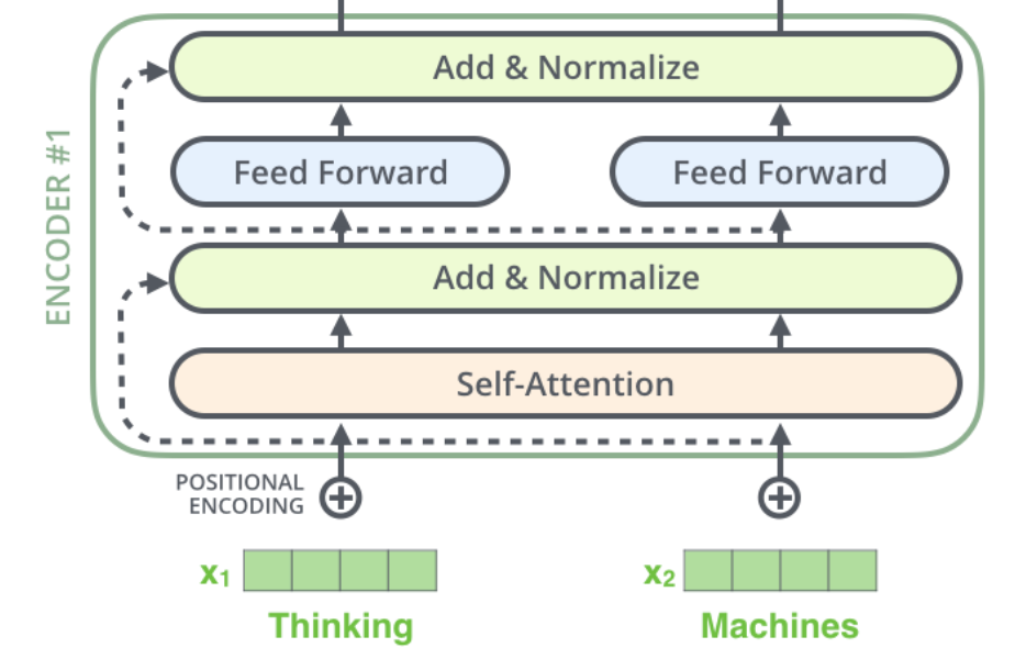

2.3.2 LayerNorm and Residual Connection

As shown above, "Add" represents the residual connection, and "Norm" represents LayerNorm. The output from the self-attention layer, Self-Attention(Q, K, V), is added to the model’s input, X_embedding, for residual connection: $$ X_{embedding} + Self-Attention(Q, K, V) $$ The result of the residual connection is then layer-normalized. Layer normalization standardizes the hidden layer to a standard normal distribution, which accelerates the training process and helps the model converge faster.

The steps for Layer Normalization are as follows:

1. Compute Mean $\mu_i$： $$ \mu_i = \frac{1}{D} \sum_{j=1}^{D} x_{ij} $$

​ For an input $X$ with a shape of [B, S, D], the mean is computed along the last dimension.

2. Compute Variance $\sigma_i^2$： $$ \sigma_i^2 = \frac{1}{D} \sum_{j=1}^{D} (x_{ij} - \mu_i)^2 $$

3. Normalize Each Sample's Features: $$ \hat{x}{ij} = \frac{x{ij} - \mu_i}{\sqrt{\sigma_i^2 + \epsilon}} $$

​ Where $\epsilon$ is a small constant, usually $10^{-5}$ or $10^{-6}$, to prevent division by zero.

4. Apply Scaling and Shifting (Learnable Parameters $\gamma$ and $\beta$)： $$ y_{ij} = \gamma \hat{x}_{ij} + \beta $$

   Here, $\gamma$ and $\beta$ are learnable parameters, with dimensions matching the input $X$'s dimension $D$. These parameters are learned during training, allowing the network to restore the original representation space. During inference, these parameters can be accessed in the model’s weights.

The final output, $y_{ij}$, is the result of layer normalization and will be used as input for the next layer or operation.

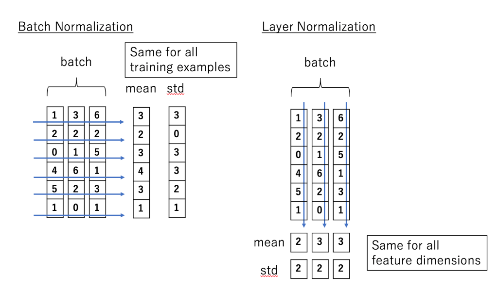
The diagram above illustrates the difference between Batch Normalization and Layer Normalization. The key difference is that Layer Normalization normalizes each data point individually, without considering others, thus avoiding the impact of different batch sizes.

In PyTorch, LayerNorm can be easily applied using the following API:

self.norm2 = nn.LayerNorm(d_model)

2.3.3 Feed Forward Network (FFN)

The FFN, or Feed Forward Neural Network, is designed to introduce non-linearity, helping the model learn more complex representations. The FFN consists of the following steps:

• Linear Transformation: The input first undergoes a linear transformation, mapping its dimension from d_model to a larger dimension d_ff. Typically, d_ff is four times d_model.
• Activation Function: A non-linear activation function, such as ReLU or GeLU (Gaussian Error Linear Unit), is applied to enhance the model’s expressive power.
• Second Linear Transformation: The activated result is then passed through another linear transformation, mapping the dimension back from d_ff to d_model.

class FeedForwardNetwork(nn.Module):
    def __init__(self):
        super(FeedForwardNetwork, self).__init__()
        self.fc1 = nn.Linear(d_model, d_ff)
        self.fc2 = nn.Linear(d_ff, d_model)

        self.gelu = gelu

    def forward(self, x):
        x = self.fc1(x)
        x = self.gelu(x)
        x = self.fc2(x)
        return x

This approach allows the FFN to capture complex patterns and dependencies in the input data.

2.4 Model Parameters and Size

BERT’s key parameters are defined as follows:

max_len = 30
max_vocab = 50
max_pred = 5

d_k = d_v = 64
d_model = 768  # n_heads * d_k
d_ff = d_model * 4

n_heads = 12
n_layers = 6
n_segs = 2

• max_len: The maximum length of the input sequence.
• max_vocab: The maximum size of the vocabulary.
• max_pred: The maximum number of tokens that can be masked during training.
• d_k, d_v: The dimensions of the Key and Value in self-attention, with the dimension of the Query equal to that of the Key since they must always be equal.
• d_model: The size of the Embedding.
• d_ff: The hidden layer size of the Feed Forward Network, generally four times d_model.
• n_heads: The number of heads in multi-head attention.
• n_layers: The number of stacked Encoder layers.
• n_segs: The number of sentence segments for segment embedding in BERT.

The diagram below shows the architecture of the original BERT models, highlighting the differences between BERT Base and BERT Large:

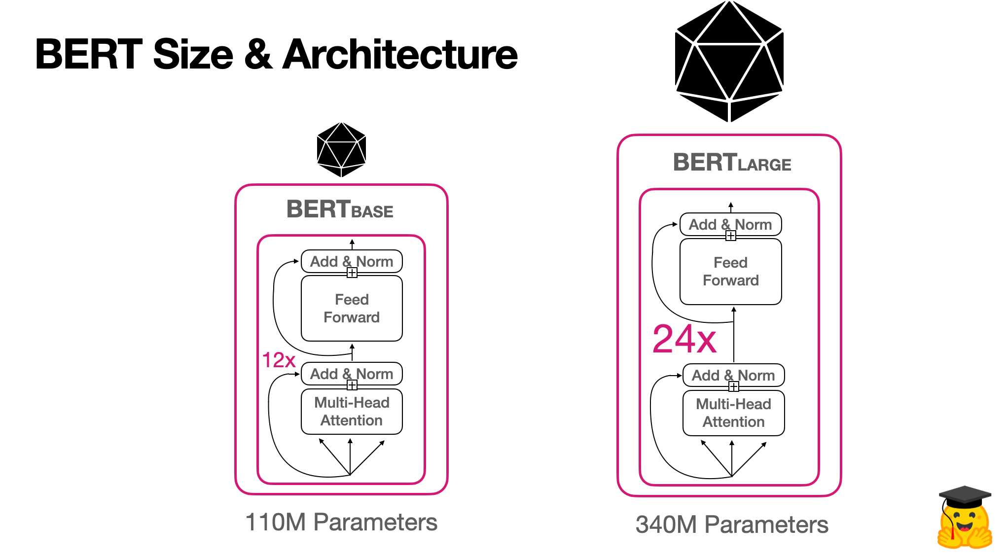
The table below further illustrates the differences in parameters between the commonly used BERT Base and BERT Large models:

3. Inference Optimization of BERT

3.1 Torch Inference Implementation

The following code natively implements a classification network based on BERT. By assembling the various modules mentioned earlier, we construct the Encoder Layer and then build the entire network structure.

Previously, we didn't get into the shape transformations of tensors during computation. In the code below, these transformations are annotated. Different operations lead to different shape changes, which is a detailed aspect of the implementation:

maxlen = 30  # Maximum length of the input sequence.
batch_size = 6
max_pred = 5  # Maximum number of tokens for prediction in the vocabulary.
n_layers = 6  # Number of stacked Encoder layers.
n_heads = 12  # Number of attention heads.
d_model = 768  # Size of the embedding (n_heads * d_k).
d_ff = 768 * 4  # 4 * d_model, the hidden layer size of the Feed Forward Network, typically four times d_model.
d_k = d_v = 64  # Dimension of K(=Q) and V in self-attention. The dimension of Q is set equal to K since they must always match.
n_segments = 2  # Number of sentence segments input into BERT, used for creating Segment Embeddings.

class Embedding(nn.Module):
    def __init__(self):
        super(Embedding, self).__init__()
        self.tok_embed = nn.Embedding(vocab_size, d_model)  # token embedding
        self.pos_embed = nn.Embedding(maxlen, d_model)  # position embedding
        self.seg_embed = nn.Embedding(n_segments, d_model)  # segment(token type) embedding
        self.norm = nn.LayerNorm(d_model)

    def forward(self, x, seg):
        seq_len = x.size(1)
        pos = Torch.arange(seq_len, dtype=Torch.long)
        pos = pos.unsqueeze(0).expand_as(x)  # [seq_len] -> [batch_size, seq_len]
        embedding = self.tok_embed(x) + self.pos_embed(pos) + self.seg_embed(seg)
        return self.norm(embedding)

class ScaledDotProductAttention(nn.Module):
    def __init__(self):
        super(ScaledDotProductAttention, self).__init__()

    def forward(self, Q, K, V, attn_mask):
        scores = Torch.matmul(Q, K.transpose(-1, -2)) / np.sqrt(d_k) # scores : [batch_size, n_heads, seq_len, seq_len]
        scores.masked_fill_(attn_mask, -1e9) # Fills elements of self tensor with value where mask is one.
        attn = nn.Softmax(dim=-1)(scores)
        context = Torch.matmul(attn, V)
        return context

class MultiHeadAttention(nn.Module):
    def __init__(self):
        super(MultiHeadAttention, self).__init__()
        self.W_Q = nn.Linear(d_model, d_k * n_heads)
        self.W_K = nn.Linear(d_model, d_k * n_heads)
        self.W_V = nn.Linear(d_model, d_v * n_heads)
    def forward(self, Q, K, V, attn_mask):
        # q: [batch_size, seq_len, d_model], k: [batch_size, seq_len, d_model], v: [batch_size, seq_len, d_model]
        residual, batch_size = Q, Q.size(0)
        # (B, S, D) -proj-> (B, S, D) -split-> (B, S, H, W) -trans-> (B, H, S, W)
        q_s = self.W_Q(Q).view(batch_size, -1, n_heads, d_k).transpose(1,2)  # q_s: [batch_size, n_heads, seq_len, d_k]
        k_s = self.W_K(K).view(batch_size, -1, n_heads, d_k).transpose(1,2)  # k_s: [batch_size, n_heads, seq_len, d_k]
        v_s = self.W_V(V).view(batch_size, -1, n_heads, d_v).transpose(1,2)  # v_s: [batch_size, n_heads, seq_len, d_v]

        attn_mask = attn_mask.unsqueeze(1).repeat(1, n_heads, 1, 1) # attn_mask : [batch_size, n_heads, seq_len, seq_len]
        # context: [batch_size, n_heads, seq_len, d_v], attn: [batch_size, n_heads, seq_len, seq_len]
        context = ScaledDotProductAttention()(q_s, k_s, v_s, attn_mask)
        context = context.transpose(1, 2).contiguous().view(batch_size, -1, n_heads * d_v) # context: [batch_size, seq_len, n_heads, d_v]
        output = nn.Linear(n_heads * d_v, d_model)(context)
        return nn.LayerNorm(d_model)(output + residual) # output: [batch_size, seq_len, d_model]

class PoswiseFeedForwardNet(nn.Module):
    def __init__(self):
        super(PoswiseFeedForwardNet, self).__init__()
        self.fc1 = nn.Linear(d_model, d_ff)
        self.fc2 = nn.Linear(d_ff, d_model)

    def forward(self, x):
        # (batch_size, seq_len, d_model) -> (batch_size, seq_len, d_ff) -> (batch_size, seq_len, d_model)
        return self.fc2(gelu(self.fc1(x)))
class EncoderLayer(nn.Module):
    def __init__(self):
        super(EncoderLayer, self).__init__()
        self.enc_self_attn = MultiHeadAttention()
        self.pos_ffn = PoswiseFeedForwardNet()

    def forward(self, enc_inputs, enc_self_attn_mask):
        enc_outputs = self.enc_self_attn(enc_inputs, enc_inputs, enc_inputs, enc_self_attn_mask) # enc_inputs to same Q,K,V
        enc_outputs = self.pos_ffn(enc_outputs) # enc_outputs: [batch_size, seq_len, d_model]
        return enc_outputs

class BERT(nn.Module):
    def __init__(self):
        super(BERT, self).__init__()
        self.embedding = Embedding()
        self.layers = nn.ModuleList([EncoderLayer() for _ in range(n_layers)])
        self.fc = nn.Sequential(
            nn.Linear(d_model, d_model),
            nn.Dropout(0.5),
            nn.Tanh(),
        )
        self.classifier = nn.Linear(d_model, 2)
        self.linear = nn.Linear(d_model, d_model)
        self.activ2 = gelu
        # fc2 is shared with embedding layer
        embed_weight = self.embedding.tok_embed.weight
        self.fc2 = nn.Linear(d_model, vocab_size, bias=False)
        self.fc2.weight = embed_weight

    def forward(self, input_ids, segment_ids, masked_pos):
        output = self.embedding(input_ids, segment_ids) # [bach_size, seq_len, d_model]
        enc_self_attn_mask = get_attn_pad_mask(input_ids, input_ids) # [batch_size, maxlen, maxlen]
        for layer in self.layers:
            # output: [batch_size, max_len, d_model]
            output = layer(output, enc_self_attn_mask)
        # it will be decided by first token(CLS)
        h_pooled = self.fc(output[:, 0]) # [batch_size, d_model]
        logits_clsf = self.classifier(h_pooled) # [batch_size, 2] predict isNext

        masked_pos = masked_pos[:, :, None].expand(-1, -1, d_model) # [batch_size, max_pred, d_model]
        h_masked = Torch.gather(output, 1, masked_pos) # masking position [batch_size, max_pred, d_model]
        h_masked = self.activ2(self.linear(h_masked)) # [batch_size, max_pred, d_model]
        logits_lm = self.fc2(h_masked) # [batch_size, max_pred, vocab_size]
        return logits_lm, logits_clsf
model = BERT()

The above implementation is native, but there are also some libraries, such as transformers, that provide a simplified interface for BERT, making it very easy to use directly.

from transformers import BERTTokenizer, BERTForMaskedLM
tokenizer = BERTTokenizer.from_pretrained(BERT_PATH)
model = BERTForMaskedLM.from_pretrained(BERT_PATH, return_dict = True)

3.2 Operator Execution Process

Previously, we analyzed the network structure of BERT, where the core component is the Transformer’s Encoder layer. Therefore, our focus is primarily on the construction, deployment, and optimization of the Encoder layer.

First, let’s organize the operator computation process in the Encoder layer:

1. Tokenizer and Embedding $$ X = Tokenizer(text) \ X = PositionalEmbeddings(X) + TokenEmbedding(X) + SegmentEmbedding(X) \ X.shape = [B, S, D] $$

2. Self-Attention $$ Q = Linear_q(X) \ K = Linear_k(X) \ V = Linear_v(X)\ X_{attention} = \text{Softmax}\left(\frac{QK^T}{\sqrt{d_k}}\right)V $$ (If it’s Multi-head Attention, there is an additional Linear layer afterward.)

3. Residual Connection and Layer Norm $$ X_{attention} = X_{attention} + X \ X_{attention} = Layer Norm(X_{attention}) $$

4. FFN, Residual Connection, and Layer Norm $$ X_{hidden} = Linear(ReLU(Linear(X_{attention}))) \ X_{hidden} = X_{attention} + X_{hidden} \ X_{hidden} = LayerNorm(X_{hidden}) $$

We can see that there are five types of operators: Embedding, Linear, Softmax, LayerNorm, and ReLU. Among them, the most time-consuming is the Linear layer, which involves matrix multiplication.

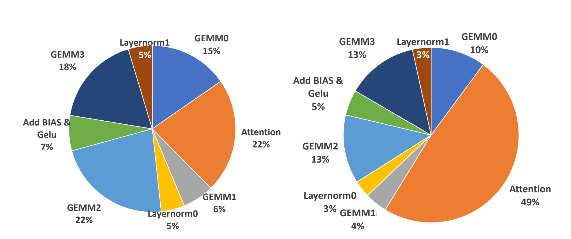
The specific operator execution flow is illustrated in the figure below:

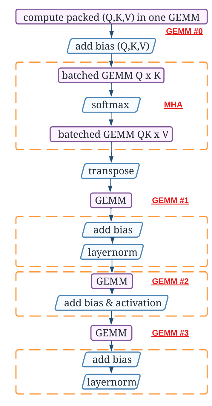
GEMM0 to GEMM3 refer to four consecutive matrix multiplications (GEMM stands for General Matrix Multiply), and they are numbered from GEMM #0 to GEMM #3 in the diagram above. The other two Batched GEMMs are part of the Self-Attention (the reason for using Batched GEMM is that multi-head attention has multiple groups of computations, which can be batch processed to improve efficiency), and thus, along with Softmax, are collectively referred to as MHA (Multi-Head Attention) in the diagram.

The following figure shows the profile of the Encoder layer under two sequence lengths (left: 256, right: 1024). Performance analysis results indicate that computation-intensive GEMM operations account for 61% and 40% of the total execution time in the two test cases, respectively. The Attention module, including a Softmax and two Batched GEMMs, is the most time-consuming part. As the sequence length increases from 256 to 1024, the Attention module occupies 49% of the total execution time, while the remaining memory-bound operations (Layer Normalization, adding bias, and activation) only take up 11%-17%.

Given the above analysis, we can optimize the Encoder's inference by focusing on four main points: Batch GEMM, optimizing MHA, operator fusion, and Varlen. Below is a detailed introduction to each of these optimizations.

3.3 Optimization 1: Batch GEMM

In the computation process described earlier, the following three matrix multiplications occur: $$ Q = Linear_q(X) \ K = Linear_k(X) \ V = Linear_v(X) $$

These three matrices have the same shape and share the same input. Therefore, concatenating the three weight matrices together and using cuBLAS's Batched GEMM can increase bandwidth and improve computational efficiency.

Typically, matrix multiplication calls cuBLAS's cublasGemmEx. Here, cublasGemmStridedBatchedEx can be used for greater efficiency. Both are GEMM (General Matrix Multiply) interfaces provided by NVIDIA's cuBLAS. The main differences between the two are as follows:

1. cublasGemmEx：

This function is used for general matrix multiplication, i.e. $C = α × A × B + β × C$。This function can perform computations on input matrices with different precisions and data types. It is commonly used for a single matrix multiplication operation. This interface has the advantage of high-performance computation using different precisions and mixed data types.

2. cublasGemmStridedBatchedEx:

This function performs batched matrix multiplication, i.e., completing all matrix multiplication operations at once given a set of matrices (referred to as a batch). Each batch's matrix multiplication is calculated as $C_i = α × A_i × B_i + β × C_i$, where $A_i$、$B_i$ and $C_i$ are the input and output matrices for each batch. It uses a mechanism called "strided" memory layout, meaning that the input matrices $A_i$, $B_i$ and output matrices $C_i$ are stored in contiguous blocks in memory, with a fixed stride between each consecutive block. This can generally improve memory access and computational performance.

This optimization requires concatenating $W^Q$, $W^K$, $W^V$ (i.e., the model weights) together and ensuring they are contiguous in GPU memory.

3.4 Optimization 2: MHA

In the Self-Attention, operator fusion can also be applied. The following operations can all be fused into one operator: $$ Q = Linear_q(X) \ K = Linear_k(X) \ V = Linear_v(X)\ X_{attention} = \text{Softmax}\left(\frac{QK^T}{\sqrt{d_k}}\right)V $$ There are two reasons for this optimization: first, Attention is very memory-intensive, as $QK^T$​ has a shape of $[B, N, S, S]$, which can be very memory-consuming when S is large; the second reason is that this operation is memory-bound, meaning it cannot fully utilize computational resources. There are various optimization methods, including TensorRT’s MHA, Flash-Attention, and xformers' memory_efficient_attention. Below is a brief introduction to these three Attention optimizations.

These three Attention mechanisms are all designed to optimize the Multi-Head Attention (MHA) computation in Transformer models. They each take different approaches to improving efficiency, reducing memory usage, or accelerating computation.

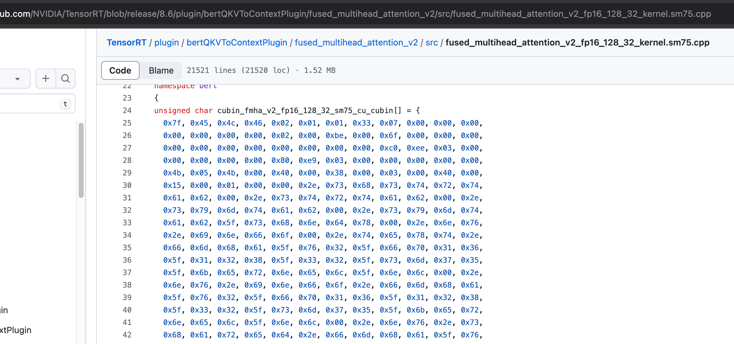
1. TensorRT's MHA:

• TensorRT’s MHA optimization may include techniques like kernel fusion, precision calibration, and automatic layer adjustment to reduce latency and memory usage when executing multi-head self-attention.
• TensorRT's MHA has multiple versions, all provided as open-source binaries. Various binary files are compiled based on different machines and needs and placed into a Plugin. The native implementation is not visible.
• To use it, you can compile the TensorRT Plugin and insert it into your project.
  • 

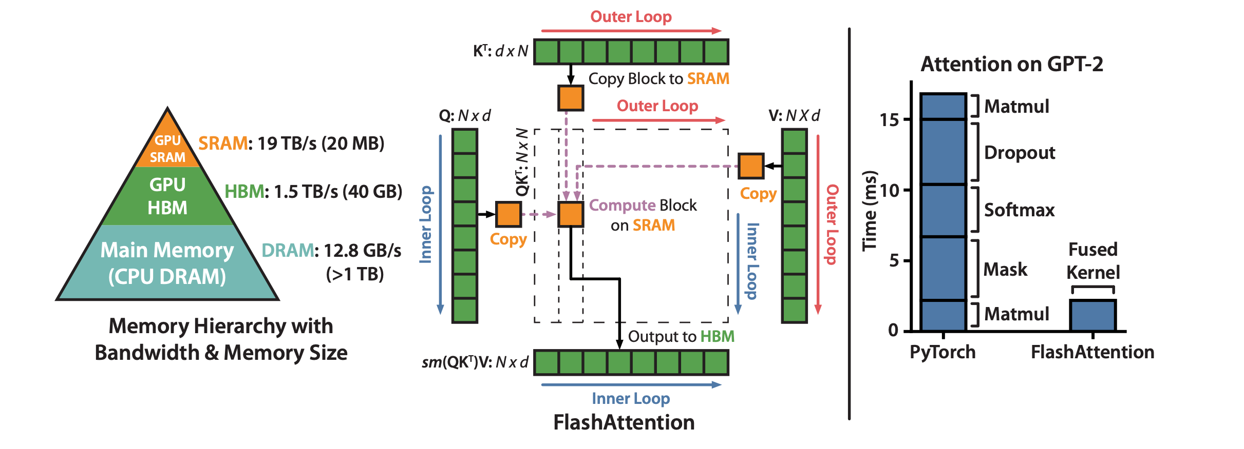
2. Flash-Attention:

   • Flash-Attention is a technique designed to accelerate self-attention computation in Transformer models. It improves efficiency by reducing global synchronization points and optimizing memory access patterns. Flash-Attention specifically focuses on reducing memory usage during attention computation on large models and long sequences, enabling large models to run on limited hardware resources. It is designed for efficient self-attention computation on NVIDIA GPUs.

   • Code：https://github.com/Dao-AILab/flash-attention Paper：https://arxiv.org/abs/2205.14135

   • In simple terms, Flash-Attention fully utilizes the GPU's memory architecture by tiling the input and placing it into faster-shared memory and registers, ensuring data is constantly stored in faster memory devices. Additionally, the operations of $QK^T$ and row-wise Softmax computation are fused. This not only fully utilizes computational resources but also reduces the memory usage of the large attention scores $[B, N, S, S]$, meaning memory usage now grows linearly, allowing for training and inference with longer sequence lengths.

   • Flash-Attention has two versions, Flash-Attention1 and Flash-Attention2. Version 2 is optimized in terms of computation compared to version 1, resulting in faster speeds.

   • To use, you can directly call or modify the open-source repository, or use Torch 2.0 and above versions. Torch’s torch.nn.functional.scaled_dot_product_attention already implements Flash-Attention2, so you can call it directly, or compile it from the source repository as a TensorRT Plugin and insert it into your project.

     

3. xformers' memory_efficient_attention:

   • xformers is a modular Transformer library that provides various components to improve the efficiency of Transformer models. memory_efficient_attention is a feature in xformers that implements a memory-efficient attention mechanism. This mechanism reduces memory usage during attention operations by employing a recomputation strategy and optimized data layout. This is particularly useful for training large models, as it allows for training larger models or using longer sequences on a single GPU.
   • Code：https://github.com/facebookresearch/xformers Paper：https://arxiv.org/pdf/2112.05682
   • In directions like SD and SVD, xformers' memory_efficient_attention usually performs better.
   • To use, you can call it from xformers, or Torch’s torch.nn.functional.scaled_dot_product_attention (though it’s implemented slightly differently in xformers). This function implements three types of attention and automatically selects the attention implementation based on the input shape.

3.5 Optimization 3：Kernel fusion

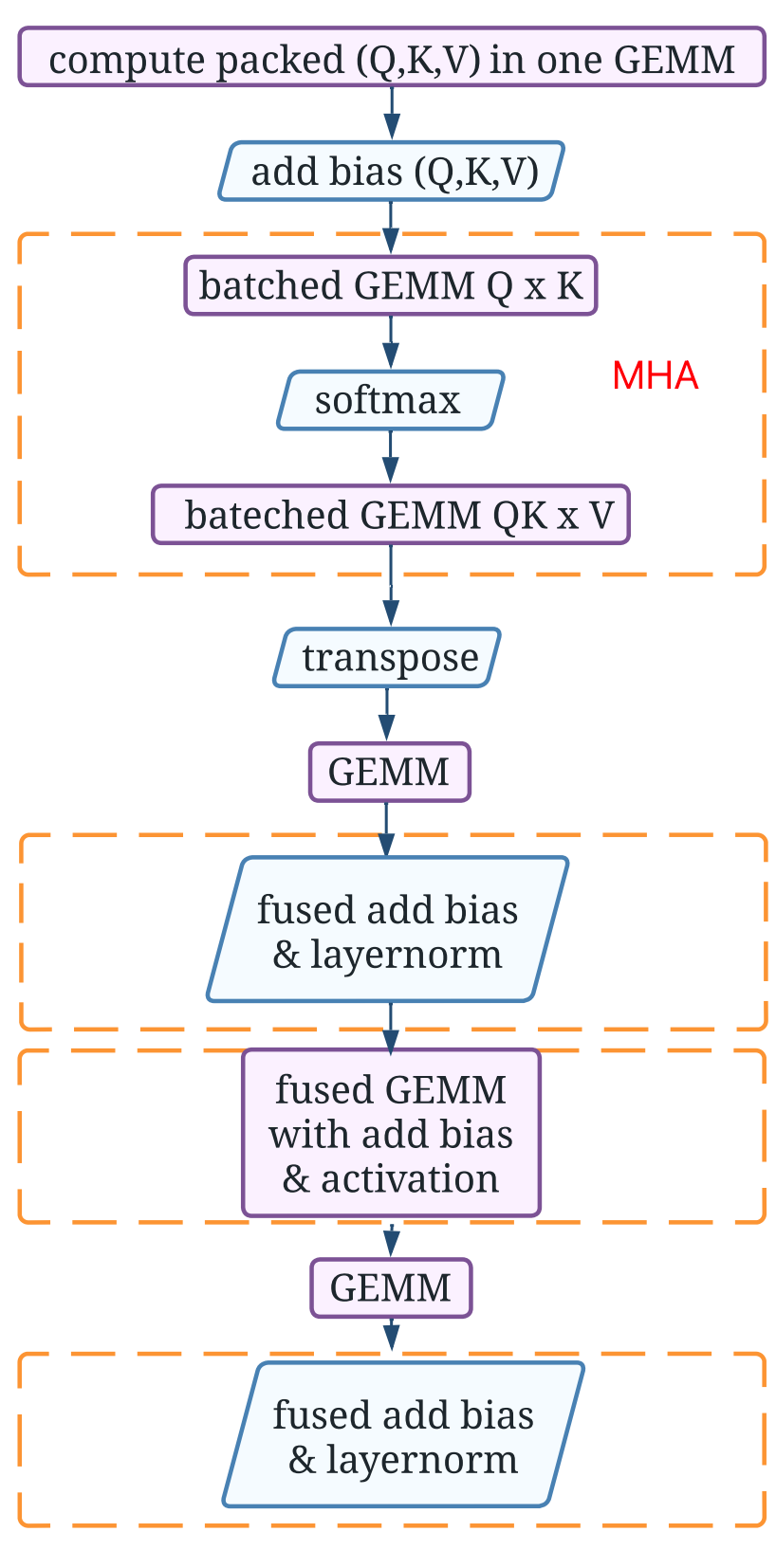
Kernel fusion primarily involves two types of operations: the fusion of Add Bias and Layer Norm, and the fusion of GEMM with Add Bias and Activation. The essence of operator fusion is to reduce the time spent on memory access by combining computational operations to minimize memory access frequency or to perform computations in faster storage.

Add bias & Layer norm

As seen in the operator execution diagram above, there are matrix multiplications preceding the two layer norm operations, and matrix multiplication usually involves bias. By fusing the add bias operation with layer norm, we can achieve higher efficiency.

From the profile above, these operations account for 10% and 6% of the total execution time when the sequence lengths are 256 and 1024, respectively. The general implementation involves two rounds of memory access to load and store the tensors. By implementing operator fusion in the kernel, only one round of global memory access is needed to complete layer normalization and bias addition. This sub-kernel's fusion improved performance by 61%, which, correspondingly, increased the performance of a single-layer BERT transformer by an average of 3.2% for sequence lengths between 128 and 1024 (data from ByteTransformer).

GEMM with add bias & Activation

Add bias and activation: For sequence lengths of 256 and 1024, these operations account for 7% and 5% of the total execution time, respectively. After matrix multiplication projection, the result tensor is added to the input tensor and then element-wise activated using the GELU activation function. The fusion implementation here does not store the output of the GEMM (General Matrix Multiply) to global memory and then reload it for adding bias and activation. Instead, it reuses the GEMM result matrix at the register level by implementing a customized fused CUTLASS. Here, the GEMM perfectly hides the memory latency of bias addition and GELU activation entering the GEMM. As a result, the performance of a single-layer BERT was improved by about 3.8%.

The following figure shows the operator execution diagram after kernel fusion. You can see two Add Bias & Layer Norm and one GEMM with Add Bias & Activation, each implemented using a single operator rather than multiple operators as before.

3.6 Optimization 4：Varlen

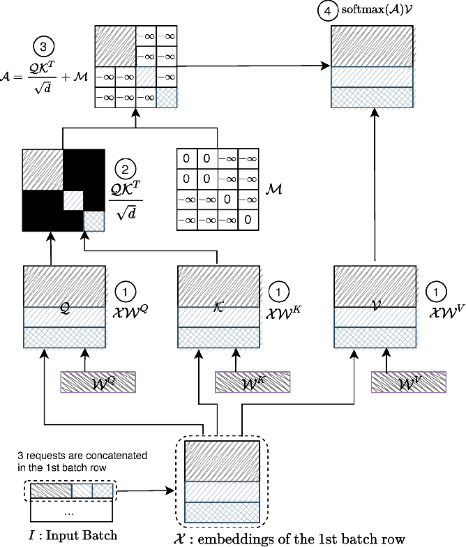
This optimization targets service scenarios with numerous requests where the input sizes vary significantly. Typically, these requests are batched, and the sequence length dimension S is padded to match the length of the longest input in the batch. If the variance in input length is large, this can lead to redundant computations. Varlen addresses this issue in such scenarios.

There are two approaches: one is to concatenate all inputs into a single sequence, set the batch size to 1, and use a prefix sum to mark the data length. The other approach involves multiple batches but with more complex markings.

TensorRT

The following diagram illustrates the first approach. This method is mentioned in both TensorRT and TCB. In the Transformer Encoder Layer, most operators depend on the last dimension D, while here, the first two dimensions [B, S] are modified. Therefore, only the operators affected by the first two dimensions need to be modified. This mainly impacts the Mask and Softmax operations in the Attention mechanism. The Mask implementation differs from the original, as shown in the diagram below, where the mask region changes and the Softmax operation also changes slightly. Everything else remains the same.

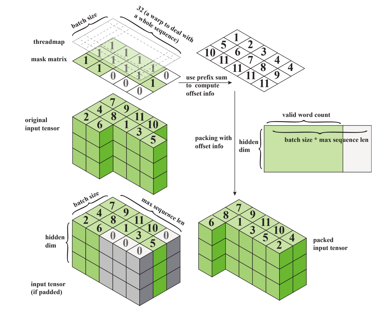
ByteTransformer

Another implementation is proposed by ByteTransformer, which is more complex but offers better performance. As seen in the padding mechanism diagram below, an array is needed to mark the position of each input. Compared to the first method, which simply concatenates into one dimension, the subsequent processing will differ. It was mentioned earlier that the Attention implementation is affected in the Encoder Layer. The first method only requires modifying the mask and Softmax processing. However, the ByteTransformer method cannot be achieved by simply modifying the mask.

ByteTransformer has two versions. The first version restores the concatenated output to the padding mode during Attention processing, which is inefficient and still involves a lot of redundant computation. The second version optimizes this by improving Group GEMM in Cutlass, allowing simultaneous computation of multiple matrices of different sizes.

4. BERT Inference Optimization with TensorRT

TensorRT is a high-performance deep learning inference platform provided by NVIDIA, specifically designed for production environments. TensorRT can significantly enhance the speed, efficiency, and performance of deep learning models on NVIDIA GPUs. It includes an optimizer and a runtime environment that can convert trained deep learning models into optimized inference engines. This process involves various optimization strategies such as layer and tensor fusion, kernel auto-tuning, and precision calibration. TensorRT supports three precision modes: FP32, FP16, and INT8, and provides precision calibration tools to ensure that model accuracy is maintained even when precision is reduced to improve performance. Additionally, TensorRT supports dynamic input, which can handle input tensors of varying sizes, making it particularly useful for processing images of different resolutions or sequences of varying lengths. If standard layers are insufficient to cover specific model needs, TensorRT offers a plugin API that allows developers to create custom layers.

Unfortunately, TensorRT is currently only available on NVIDIA GPUs and cannot be applied to other manufacturers' GPUs. Other major manufacturers have also launched inference platforms tailored to their GPUs.

Next, we will use TensorRT to optimize BERT inference. This section introduces two methods for converting a model to TensorRT: one using the TensorRT API for network construction and the other using ONNX for conversion. Additionally, it covers how to write a TensorRT Plugin and use it in a network, as well as how to accelerate using FP16 and INT8 in TensorRT.

4.1 Overview of the TensorRT Workflow

The general steps for building TensorRT are as follows:

Step 1: Create a logger Step 2: Create a builder Step 3: Create a network Step 4: Add layers to the network Step 5: Set and mark the output Step 6: Create a config and set the maximum batch size and workspace size Step 7: Create an engine Step 8: Serialize and save the engine Step 9: Release resources

An example is shown in the following code:

import TensorRT as trt

logger = trt.Logger(trt.Logger.ERROR)

builder = trt.Builder(logger)
builder.reset()  # reset Builder as default, not required

network = builder.create_network(1 << int(trt.NetworkDefinitionCreationFlag.EXPLICIT_BATCH))
config = builder.create_builder_config()
inputTensor = network.add_input("inputT0", trt.float32, [3, 4, 5])
identityLayer = network.add_identity(inputTensor)
network.mark_output(identityLayer.get_output(0))
builder.max_batch_size = 8
builder.max_workspace_size = 1 << 30
engineString = builder.build_serialized_network(network, config)

The most labor-intensive part is building the network. Depending on the network, you need to use the corresponding operators to construct it, and then follow the process to build the engine.

There are two main ways to build a network: using the TensorRT API or converting from ONNX. Each method has its pros and cons, as outlined below:

Building the Network Directly Using the TensorRT API:

Advantages:

• Direct use of the TensorRT API allows full utilization of all TensorRT optimization features, including layer fusion, precision mixing (FP32, FP16, INT8), etc.
• You can manually adjust and optimize the parameters and configurations of each layer to achieve the best performance.
• You have complete control over every layer and operation in the network, making it suitable for highly customized application scenarios.
• You can directly use various advanced features and plugins provided by TensorRT.
• You can finely control memory allocation, data flow, and the execution order of the computation graph, which is ideal for applications with extremely high-performance requirements.

Disadvantages:

• Requires deep understanding of the TensorRT API and low-level implementation, making development and debugging more complex.
• For complex network structures, manual coding can be very tedious and error-prone.
• Code written directly with the TensorRT API is usually tied to specific hardware and software environments, and porting to other platforms may require significant modifications.
• Due to the high level of customization in the code, the maintenance and update costs can be high.

Parsing TensorRT Networks Using ONNX:

Advantages:

• You can use high-level deep learning frameworks (such as PyTorch, TensorFlow) to build and train models, then export them in ONNX format.
• ONNX models can be directly imported into TensorRT, simplifying the development process.
• ONNX is an open standard format that supports multiple deep learning frameworks and hardware platforms.
• Using ONNX makes it easier to port models across different platforms.
• ONNX has broad community support and a rich ecosystem of tools, allowing you to leverage existing tools for model conversion, optimization, and deployment.
• Building and training models with high-level frameworks results in more concise code and lower maintenance costs.

Disadvantages:

• Although TensorRT optimizes ONNX models, the performance may not match that of manual optimization.
• Some advanced optimizations and custom operations may not be expressible through ONNX, requiring additional plugins or manual adjustments.
• You need to ensure that the deep learning framework you're using and TensorRT both support the ONNX format.
• Some new features or custom layers may not be supported in ONNX, leading to model conversion failures or performance degradation.
• If problems occur when importing an ONNX model, debugging can be more complicated, requiring knowledge of both the ONNX format and TensorRT's internal implementation.

In summary:

• Building Networks Directly Using the TensorRT API: suitable for application scenarios requiring high customization and performance optimization, but the development and maintenance costs are high.
• Parsing TensorRT Networks Using ONNX: suitable for scenarios where simplifying the development process, improving cross-platform compatibility, and reducing maintenance costs are priorities, though there may be trade-offs in performance and flexibility.

Which method to choose depends on the specific application needs, development resources, and performance requirements. For most applications, using ONNX to parse TensorRT networks is a more straightforward and efficient choice, while for applications requiring extreme performance optimization, direct use of the TensorRT API can be considered.

4.2 Building BERT Using API

Typically, networks are built using Torch, but when using TensorRT for inference, you need to build the network using its API, which differs significantly from Torch's API.

Below are some examples to introduce TensorRT's API:

Relu

def addReLU(self, layer, x, layer_name=None, precision=None):
    trt_layer = self.network.add_activation(x, type=trt.ActivationType.RELU)

    if layer_name is None:
        layer_name = "nn.ReLU"

    self.layer_post_process(trt_layer, layer_name, precision)

    x = trt_layer.get_output(0)
    return x

In the code above, a ReLU activation layer is added by calling TensorRT's self.network.add_activation, with the activation type set to trt.ActivationType.RELU. TensorRT supports various activation functions such as trt.ActivationType.TANH, and different types can be selected by setting the appropriate type.

The layer_post_process function is then used to set the layer name (which is helpful during debugging and building processes) and to check the shape. Finally, the output of this layer is obtained using trt_layer.get_output(0) and returned.

Reshape

def addReshape(self, x, reshape_dims, layer_name=None, precision=None):
    trt_layer = self.network.add_shuffle(x)
    trt_layer.reshape_dims = reshape_dims

    if layer_name is None:
        layer_name = "Torch.reshape"
    else:
        layer_name = "Torch.reshape." + layer_name

    self.layer_post_process(trt_layer, layer_name, None)

    x = trt_layer.get_output(0)
    return x

Reshape in TensorRT is implemented using the self.network.add_shuffle API, and you need to set the target shape through trt_layer.reshape_dims. This is quite different from how reshaping is done in Torch. The subsequent steps are similar, involving post-processing and returning the output of the layer.

Linear

def addLinear(self, x, weight, bias, layer_name=None, precision=None):
    input_len = len(x.shape)
    if input_len < 3:
        raise RuntimeError("addLinear x.shape.size must >= 3")

    if layer_name is None:
        layer_name = "nn.Linear"

    # calc pre_reshape_dims and after_reshape_dims
    pre_reshape_dims = trt.Dims()
    after_reshape_dims = trt.Dims()
    if input_len == 3:
        pre_reshape_dims = (0, 0, 0, 1, 1)
        after_reshape_dims = (0, 0, 0)
    elif input_len == 4:
        pre_reshape_dims = (0, 0, 0, 0, 1, 1)
        after_reshape_dims = (0, 0, 0, 0)
    elif input_len == 5:
        pre_reshape_dims = (0, 0, 0, 0, 0, 1, 1)
        after_reshape_dims = (0, 0, 0, 0, 0)
    else:
        raise RuntimeError("addLinear x.shape.size >5 not support!")

    # add pre_reshape layer
    trt_layer = self.network.add_shuffle(x)
    trt_layer.reshape_dims = pre_reshape_dims

    self.layer_post_process(trt_layer, layer_name+"_pre_reshape", precision)

    x = trt_layer.get_output(0)

    # add Linear layer
    out_features = weight.shape[1]
    weight = trt.Weights(weight)
    if bias is not None:
        bias = trt.Weights(bias)

    trt_layer = self.network.add_fully_connected(x, out_features, weight, bias)
    self.layer_post_process(trt_layer, layer_name, precision)
    x = trt_layer.get_output(0)

    # add after_reshape layer
    trt_layer = self.network.add_shuffle(x)
    trt_layer.reshape_dims = after_reshape_dims
    self.layer_post_process(trt_layer, layer_name+"_after_reshape", precision)
    x = trt_layer.get_output(0)

    return x

The code first checks whether the input tensor x has at least 3 dimensions, as fully connected layers require at least a batch dimension and two feature dimensions (e.g., batch size, number of features). If no layer name is provided, it defaults to "nn.Linear". The function uses trt.Dims() to get the dimensionality information of the input. Based on the input tensor's dimensions, the function calculates the reshaping dimensions needed before and after the fully connected layer. This ensures that the fully connected layer can properly process the input data.

Before adding the fully connected layer, the code first adds a shuffle layer (self.network.add_shuffle) to change the shape of the input tensor to match the requirements of the fully connected layer. Then, it adds a fully connected layer (self.network.add_fully_connected), using the provided weight and bias parameters. After the fully connected layer, another shuffle layer is added to reshape the output tensor back to its original dimensions (or to a shape suitable for subsequent operations).

Additional operators like Softmax and Add are implemented similarly. The same principles apply: you can reference TensorRT's API to call these functions, passing in or setting the appropriate parameters.

Let's now build a block using the above operators, taking the Self-Attention mechanism from the Encoder as an example.

def self_attention_layer(network_helper, prefix, config, weights_dict, input_tensor, imask):
    num_heads = config.num_attention_heads
    head_size = config.head_size

    q_w = weights_dict[prefix + "attention_self_query_kernel"]
    q_b = weights_dict[prefix + "attention_self_query_bias"]
    q = network_helper.addLinear(input_tensor, q_w, q_b)
    q = network_helper.addShuffle(q, None, (0, -1, num_heads, head_size), (0, 2, 1, 3), "att_q_view_transpose")

    k_w = weights_dict[prefix + "attention_self_key_kernel"]
    k_b = weights_dict[prefix + "attention_self_key_bias"]
    k = network_helper.addLinear(input_tensor, k_w, k_b)
    k = network_helper.addShuffle(k, None, (0, -1, num_heads, head_size), (0, 2, 3, 1), "att_k_view_and transpose")
    # k = network_helper.addShuffle(k, None, (0, -1, self.h, self.d_k), (0, 2, 3, 1), "att_k_view_and transpose")

    v_w = weights_dict[prefix + "attention_self_value_kernel"]
    v_b = weights_dict[prefix + "attention_self_value_bias"]
    v = network_helper.addLinear(input_tensor, v_w, v_b)
    v = network_helper.addShuffle(v, None, (0, -1, num_heads, head_size), (0, 2, 1, 3), "att_v_view_and transpose")

    scores = network_helper.addMatMul(q, k, "q_mul_k")

    scores = network_helper.addScale(scores, 1/math.sqrt(head_size))

    attn = network_helper.addSoftmax(scores, dim=-1)

    attn = network_helper.addMatMul(attn, v, "matmul(p_attn, value)")

    attn = network_helper.addShuffle(attn, (0, 2, 1, 3), (0, -1, num_heads * head_size), None, "attn_transpose_and_reshape")

    return attn

The code first uses the addLinear function to generate the Q, K, and V matrices. These matrices are calculated by multiplying the input tensor with weight matrices and adding biases, where the weight matrices are loaded from the model weights and stored in the weights_dict dictionary. The corresponding weights are retrieved using the appropriate key. Additionally, TensorRT weights are typically loaded using NumPy arrays.

The addShuffle function is then used to reshape the Q, K, and V matrices so that they can be split into multiple heads, which is a key part of the multi-head attention mechanism. The reshaping operation here divides each matrix into num_heads, with each head having a size of head_size.

The code uses the addMatMul function to compute the dot product of Q and K, resulting in the scores. These scores represent the attention weights that each element in the input sequence gives to other elements. The scores are then scaled by dividing by the square root of head_size. After that, the addSoftmax function is used to normalize the scores. Finally, the addMatMul function multiplies the attention weights (attn) with the value (V) matrix to get the weighted value representation.

Finally, the addShuffle function is used to reshape the output back to the original shape of the input tensor.

The code above does not fully compose an attention layer since it lacks a linear layer, as well as the residual and layer normalization layers. The following code completes the attention layer.

def self_output_layer(network_helper, prefix, config, weights_dict, hidden_states, input_tensor):
    out_w = weights_dict[prefix + "attention_output_dense_kernel"]
    out_b = weights_dict[prefix + "attention_output_dense_bias"]
    out = network_helper.addLinear(hidden_states, out_w, out_b)
    out = network_helper.addAdd(out, input_tensor)
    gamma = weights_dict[prefix + "attention_output_layernorm_gamma"]
    beta = weights_dict[prefix + "attention_output_layernorm_beta"]
    out = network_helper.addLayerNorm(out, gamma, beta)
    return out
def attention_layer(network_helper, prefix, config, weights_dict, input_tensor, imask):
    attn = self_attention_layer(network_helper, prefix, config, weights_dict, input_tensor, imask)
    out = self_output_layer(network_helper, prefix, config, weights_dict, attn, input_tensor)
    return out

The self_output_layer function constructs the output portion of the self-attention layer. Similar to the previous steps, out_w and out_b are the weights and biases retrieved from the weights_dict dictionary, used for the linear transformation (typically a fully connected layer). The result of the linear transformation is then added to the input_tensor as part of the residual connection. Lastly, the gamma and beta parameters, also retrieved from weights_dict, are used for layer normalization. A LayerNorm layer is added, and the output is returned.

The attention_layer function builds the complete self-attention layer, which includes both the self-attention computation and an output layer.

This is, of course, only part of the Transformer Encoder, focusing on the core Attention mechanism. The implementation approach for other modules is consistent with this method.

After the network is fully constructed, the build parameters are set, the network is built, and finally, the serialized engine is saved locally. Before using it, we deserialize the engine, set the input, and run inference to obtain the output.

4.3 Building BERT Using ONNX

Building BERT using ONNX is simpler compared to using the API. There are two main steps: first, converting the Torch model to ONNX, and second, converting the ONNX model to a TensorRT engine.

model2ONNX

from transformers import BERTTokenizer, BERTForMaskedLM
tokenizer = BERTTokenizer.from_pretrained(BERT_PATH)
model = BERTForMaskedLM.from_pretrained(BERT_PATH, return_dict = True)
text = "The capital of France, " + tokenizer.mask_token + ", contains the Eiffel Tower."
encoded_input = tokenizer.encode_plus(text, return_tensors = "pt")
model.eval()
export_model_path = BERT_PATH + "/model.ONNX"
opset_version = 12
symbolic_names = {0: 'batch_size', 1: 'max_seq_len'}
Torch.ONNX.export(model,                                            # model being run
                  args=tuple(encoded_input.values()),                 # model input (or a tuple for multiple inputs)
                  f=export_model_path,                         # where to save the model (can be a file or file-like object)
                  opset_version=opset_version,                      # the ONNX version to export the model to
                  do_constant_folding=False,                         # whether to execute constant folding for optimization
                  input_names=['input_ids',                         # the model's input names
                               'attention_mask',
                               'token_type_ids'],
                output_names=['logits'],                    # the model's output names
                dynamic_axes={'input_ids': symbolic_names,        # variable length axes
                              'attention_mask' : symbolic_names,
                              'token_type_ids' : symbolic_names,
                              'logits' : symbolic_names})
print("Model exported at ", export_model_path)

The key function here is Torch.ONNX.export, which is used to convert a Torch model into an ONNX model.

Here’s an explanation of the parameters used in this function:

• model: The BERT model to be exported.
• args: The input arguments for the model. In this case, tuple(encoded_input.values()) is used, indicating that the model’s input is a tuple containing multiple input tensors.
• f: The path where the exported model will be saved.
• opset_version: The version of the ONNX opset to use when exporting the model.
• do_constant_folding: Whether to perform constant folding optimization. Constant folding involves pre-computing constant expressions in the computation graph during export to optimize the model.
• input_names: A list of names for the model’s inputs.
• output_names: A list of names for the model’s outputs.
• dynamic_axes: Defines dynamic axes, which indicate variable-length input and output tensors.

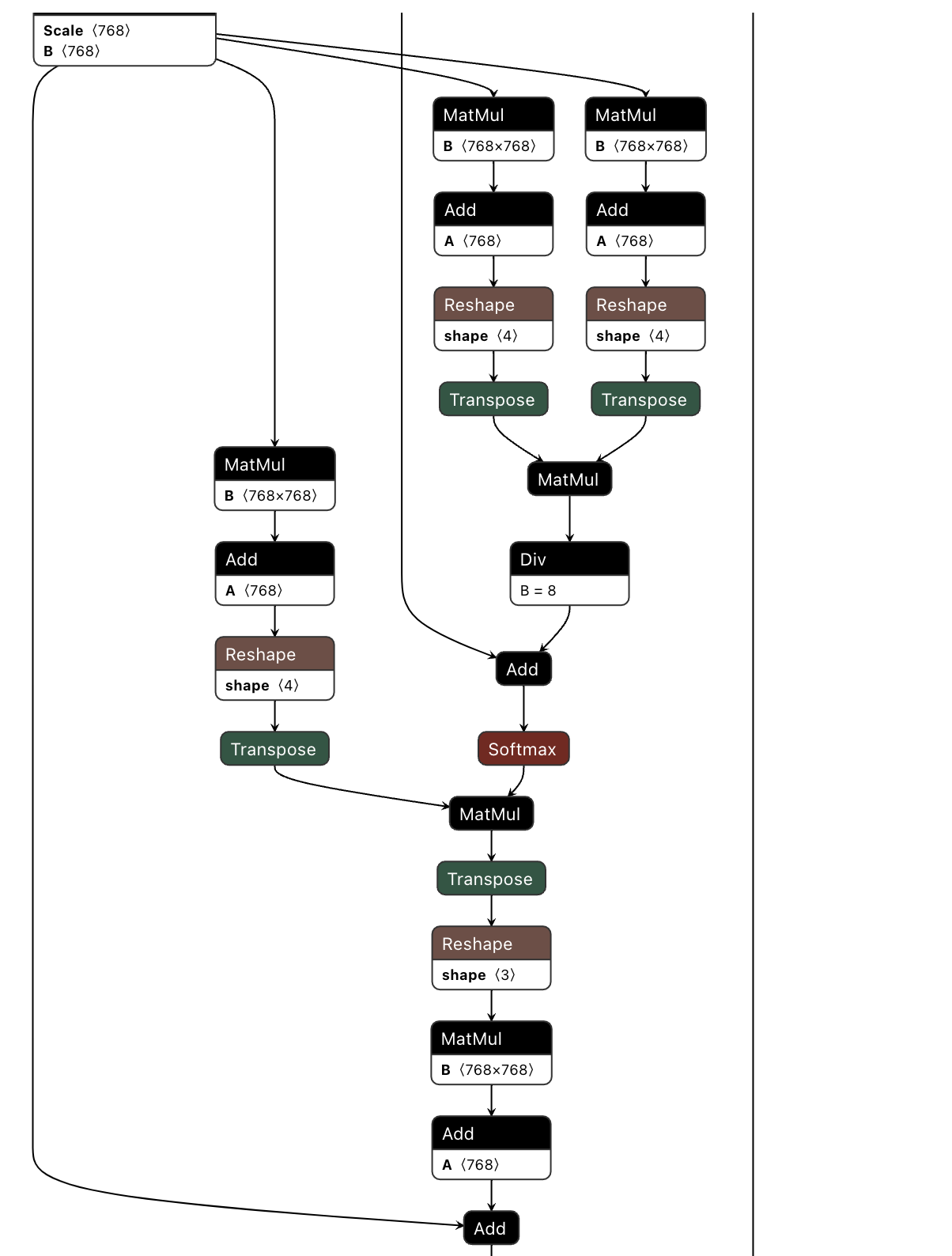
The exported ONNX model can be visualized using Netron to inspect the nodes. The image below shows some of the operators in the Self-Attention part of one layer of the BERT model. Additionally, note that the operator definitions in ONNX differ from those in Torch and TensorRT, which may lead to differences during export and conversion.

ONNX to TensorRT Conversion

There are two ways to convert an ONNX model to TensorRT: using the built-in trtexec tool or using the TensorRT API.

1. Using trtexec Command：

   trtexec is a command-line tool provided by TensorRT for quickly converting ONNX models to TensorRT engines and running inference tests.

   trtexec --ONNX=BERT.ONNX --saveEngine=BERT.engine --explicitBatch  \
           --minShapes=input_ids:1x6,token_type_ids:1x6,input_mask:1x6 \
           --optShapes=input_ids:1x64,token_type_ids:1x64,input_mask:1x64 \
           --maxShapes=input_ids:1x256,token_type_ids:1x256,input_mask:1x256
   

In this command:

• --ONNX=BERT.ONNX: Specifies the input ONNX model file.
• --saveEngine=BERT.engine: Specifies the output TensorRT engine file.
• --explicitBatch: Enables explicit batch mode.
• --minShapes, --optShapes, --maxShapes: Set the minimum, optimal, and maximum shapes for the input tensors input_ids, token_type_ids, and input_mask.

Other Common Parameters:：

• --fp16：Enables FP16 precision.
• --int8：Enables INT8 precision (requires calibration data).
• --workspace=N：Sets the maximum GPU memory workspace size (in MB).
• --batch=N：Sets the batch size.

For example, to enable FP16 precision and set the maximum workspace to 4096 MB:

trtexec --ONNX=BERT.ONNX --saveEngine=BERT.engine --explicitBatch --workspace=4096 --fp16 \
        --minShapes=input_ids:1x6,token_type_ids:1x6,input_mask:1x6 \
        --optShapes=input_ids:1x64,token_type_ids:1x64,input_mask:1x64 \
        --maxShapes=input_ids:1x256,token_type_ids:1x256,input_mask:1x256

2. Using the TensorRT API:

   def ONNX2trt(ONNXFile, plan_name):
       logger = trt.Logger(trt.Logger.VERBOSE)
   
       builder = trt.Builder(logger)
       config = builder.create_builder_config()
       profile = builder.create_optimization_profile()
       network = builder.create_network(1<<int(trt.NetworkDefinitionCreationFlag.EXPLICIT_BATCH))
       config.max_workspace_size = 3<<30
   
       parser = trt.ONNXParser(network, logger)
       print("Succeeded finding ONNX file!")
       with open(ONNXFile, 'rb') as model:
           if not parser.parse(model.read()):
               print("Failed parsing ONNX file!")
               for error in range(parser.num_errors):
                   print(parser.get_error(error))
               exit()
       print("Succeeded parsing ONNX file!")
   
       input_ids = network.get_input(0)
       token_type_ids = network.get_input(1)
       input_mask = network.get_input(2)
       profile.set_shape(input_ids.name, (1, 6), (1, 64), (1, 256))
       profile.set_shape(token_type_ids.name, (1, 6), (1, 64), (1, 256))
       profile.set_shape(input_mask.name, (1, 6), (1, 64), (1, 256))
       config.add_optimization_profile(profile)
   
       engine = builder.build_engine(network, config)
       if not engine:
           raise RuntimeError("build_engine failed")
       print("Succeeded building engine!")
   
       print("Serializing Engine...")
       serialized_engine = engine.serialize()
       if serialized_engine is None:
           raise RuntimeError("serialize failed")
   
       with open(plan_name, "wb") as fout:
           fout.write(serialized_engine

The main steps are as follows:

1. Create the core TensorRT objects, including the logger, builder, config object, optimization profile, and network object.
2. Parse the specified ONNX file and convert it into a TensorRT network representation.
3. Set the optimization profile by defining the minimum, optimal, and maximum shapes for the input tensors.
4. Build the TensorRT engine and serialize it into a byte stream.
5. Save the serialized engine to the specified file path.

4.4 Inference and Testing with TensorRT

The InferHelper class is a helper class used to load a TensorRT engine and perform inference.

class InferHelper():
    """"""
    def __init__(self, plan_name, trt_logger):
        """"""
        self.logger = trt_logger
        self.runtime = trt.Runtime(trt_logger)
        with open(plan_name, 'rb') as f:
            self.engine = self.runtime.deserialize_cuda_engine(f.read())
            self.context = self.engine.create_execution_context()
            self.context.active_optimization_profile = 0

    def infer(self, inputs: list):
        nInput = len(inputs)

        bufferD = []
        # alloc memory
        for i in range(nInput):
            bufferD.append(cuda.mem_alloc(inputs[i].nbytes))
            cuda.memcpy_htod(bufferD[i], inputs[i].ravel())
            self.context.set_binding_shape(i, tuple(inputs[i].shape))
        outputs = []
        for i in range(len(inputs), self.engine.num_bindings):
            outputs.append(np.zeros(self.context.get_binding_shape(i)).astype(np.float32))

        nOutput = len(outputs)
        for i in range(nOutput):
            bufferD.append(cuda.mem_alloc(outputs[i].nbytes))
            # print(outputs[i].nbytes)

        for i in range(len(inputs), self.engine.num_bindings):
            trt_output_shape = self.context.get_binding_shape(i)
            output_idx = i - len(inputs)
            if not (list(trt_output_shape) == list(outputs[output_idx].shape)):
                self.logger.log(trt.Logger.ERROR, "[Infer] output shape is error!")
                self.logger.log(trt.Logger.ERROR, "trt_output.shape = " + str(trt_output_shape))
                self.logger.log(trt.Logger.ERROR, "base_output.shape = " + str(outputs[output_idx].shape))
                assert(0)

        for i in range(nInput, nInput + nOutput):
            cuda.memcpy_dtoh(outputs[i - nInput].ravel(), bufferD[i])

        for i in range(0, len(outputs)):
            print("outputs.shape:" + str(outputs[i].shape))
            print("outputs.sum:" + str(outputs[i].sum()))
        return outputs

InferHelper class contains two functions: an initialization function and an inference function.

The initialization function takes plan_name, the path to the TensorRT engine file, and trt_logger, a TensorRT logger object. The steps are as follows:

1. Create a TensorRT runtime object self.runtime.
2. Open and read the TensorRT engine file.
3. Deserialize the engine file and create an engine object self.engine.
4. Create an execution context self.context.
5. Set the active optimization profile to 0.

infer method is used to perform inference, accepting a list of input tensors inputs。

The steps in the inference function are as follows:

1. Get the number of input tensors (nInput).
2. Allocate GPU memory for each input tensor and copy the data from host memory to device memory.
3. Set the shape for each input tensor.
4. Create a list of output tensors (outputs) and initialize them according to the binding shapes in the inference context.
5. Allocate GPU memory for each output tensor.
6. Check if the output shapes in the inference context match the expected output shapes. If they don't match, log an error and assert failure.
7. Copy the inference results from device memory back to host memory.
8. Print the shape and sum of the elements of the output tensors.
9. Return the list of output tensors.

With this class, you can easily perform inference using the TensorRT engine while managing the memory of input and output tensors.

Using InferHelper with BERT:

tokenizer = BERTTokenizer.from_pretrained('BERT-base-uncased')
text = "The capital of France, " + tokenizer.mask_token + ", contains the Eiffel Tower."
encoded_input = tokenizer.encode_plus(text, return_tensors = "pt")
TRT_LOGGER = trt.Logger(trt.Logger.VERBOSE)
infer_helper = InferHelper(plan_name, TRT_LOGGER)
input_list = [encoded_input['input_ids'].detach().numpy(), encoded_input['token_type_ids'].detach().numpy(), encoded_input['attention_mask'].detach().numpy()]
output = infer_helper.infer(input_list)
print(output)

In this code, a pre-trained BERT tokenizer is used to encode the input text. Then, an InferHelper object is initialized, loading the TensorRT engine. Next, the input data is prepared by converting PyTorch tensors into NumPy arrays. Finally, the InferHelper object is used to perform inference, and the inference results are printed.

Performance Testing

trtexec provides many parameters to control the performance testing behavior. Here are some commonly used parameters:

• --iterations=N：Set the number of inference iterations to run.
• --duration=N：Set the duration of the test (in seconds).
• --warmUp=N：Set the warm-up time (in seconds).
• --batch=N：Set the batch size.

Usage example:

trtexec --loadEngine=BERT.engine --batch=1 --shapes=input_ids:1x6,token_type_ids:1x6,input_mask:1x6 --fp16 --duration=60 --warmUp=10 --workspace=4096

After running the trtexec command, you will see a series of outputs, including performance metrics like average latency, throughput, etc. Here are some key metrics explained:

• Average latency: The average time per inference.
• Throughput: The number of inferences processed per second.
• Host Walltime: The total time for the entire testing process.
• GPU Compute Time: The total time spent performing inference on the GPU.

4.5 Implementing a TensorRT Plugin

In TensorRT, a Plugin is a powerful feature that allows for extending and customizing TensorRT’s capabilities. Plugins enable users to define custom layers or operations that can be used during TensorRT optimization and inference. This is particularly useful for operations not included in the standard TensorRT set or for creating custom operations.

• Custom Operations: Plugins allow users to define operations that may not exist in the standard TensorRT operations set. For example, specific activation functions, normalization operations, or other complex calculations.
• Performance Optimization: Plugins can be used to optimize the performance of specific operations. By writing efficient CUDA code, users can achieve faster computation than standard TensorRT operations.
• Support for New Models and Operations: Plugins enable TensorRT to support new model architectures and operations. As deep learning evolves rapidly with new models and operations emerging frequently, plugins provide a flexible way to support these new features.

Process of Writing and Using a TensorRT Plugin

• Defining the Plugin Class: Users need to define a class that inherits from IPluginV2 or IPluginV2DynamicExt and implement the necessary virtual functions. These functions include initialization, execution, serialization, and deserialization.
• Registering the Plugin: After defining the plugin class, it must be registered with TensorRT. This can be done using the IPluginCreator interface.
• Using the Plugin: During the construction of the TensorRT engine, the custom plugin layer can be added to the network using the INetworkDefinition interface.

The TensorRT API is available in both C++ and Python, but writing a Plugin requires C++. The kernel implementation functions need to be written in CUDA.

4.5.1 Defining a Plugin Class in TensorRT

When defining a plugin class in TensorRT, a series of key virtual functions must be implemented. These functions handle tasks such as plugin initialization, execution, serialization, and deserialization. By implementing these functions, users can create custom operations and integrate them into TensorRT’s optimization and inference processes. Below is an example of a plugin class with a series of key virtual functions.

#include "NvInfer.h"
#include "NvInferPlugin.h"

using namespace nvinfer1;

class MyCustomPlugin : public IPluginV2DynamicExt {
public:
    MyCustomPlugin() {}
    MyCustomPlugin(const void* data, size_t length) {}

    // Implement required virtual functions
    int getNbOutputs() const override { return 1; }
    DimsExprs getOutputDimensions(int outputIndex, const DimsExprs* inputs, int nbInputs, IExprBuilder& exprBuilder) override {
        return inputs[0];
    }
    int initialize() override { return 0; }
    void terminate() override {}
    size_t getWorkspaceSize(const PluginTensorDesc* inputs, int nbInputs, const PluginTensorDesc* outputs, int nbOutputs) const override { return 0; }
    int enqueue(const PluginTensorDesc* inputDesc, const PluginTensorDesc* outputDesc, const void* const* inputs, void* const* outputs, void* workspace, cudaStream_t stream) override {
        // Implement your custom operation here
        return 0;
    }
    size_t getSerializationSize() const override { return 0; }
    void serialize(void* buffer) const override {}
    void destroy() override { delete this; }
    const char* getPluginType() const override { return "MyCustomPlugin"; }
    const char* getPluginVersion() const override { return "1"; }
    IPluginV2DynamicExt* clone() const override { return new MyCustomPlugin(); }
    void setPluginNamespace(const char* PluginNamespace) override {}
    const char* getPluginNamespace() const override { return ""; }
};

Explanation of Key Functions:

1. getNbOutputs()

int getNbOutputs() const override;

• Purpose: Returns the number of outputs the plugin will produce.
• Return Value: The number of output tensors.

2. getOutputDimensions()

DimsExprs getOutputDimensions(int outputIndex, const DimsExprs* inputs, int nbInputs, IExprBuilder& exprBuilder) override;

• Purpose: Calculates and returns the dimensions of the output tensor based on the input tensor dimensions. TensorRT requires that the input and output shapes are either known or derivable.
• Parameters
  • outputIndex: he index of the output tensor.
  • inputs: The array of input tensor dimensions.
  • nbInputs: The number of input tensors.
  • exprBuilder: A tool used for constructing dimension expressions.
• Return Value: The dimensions of the output tensor.

3. getWorkspaceSize()

size_t getWorkspaceSize(const PluginTensorDesc* inputs, int nbInputs, const PluginTensorDesc* outputs, int nbOutputs) const override;

• Purpose: Returns the size of the workspace required by the plugin during execution (in bytes). If the plugin requires additional memory during inference, this function should return the size of that memory.
• Parameters
  • inputs: The array of input tensor descriptors.
  • nbInputs: The number of input tensors.T
  • outputs: The array of output tensor descriptors.
  • nbOutputs: The number of output tensors.
• Return Value: The size of the workspace in bytes.

4. enqueue()

int enqueue(const PluginTensorDesc* inputDesc, const PluginTensorDesc* outputDesc, const void* const* inputs, void* const* outputs, void* workspace, cudaStream_t stream) override;

• Purpose：Executes the plugin’s computation logic. This is the most important function, as it implements the forward inference logic for the Plugin.
• Parameters
  • inputDesc: The array of input tensor descriptors.
  • outputDesc: The array of output tensor descriptors.
  • inputs: The array of pointers to the input tensor data.
  • outputs: The array of pointers to the output tensor data.
  • workspace: A pointer to the workspace memory.
  • stream: The CUDA stream.
• Return Value: Returns 0 on success, non-zero on failure.

5. getSerializationSize()

size_t getSerializationSize() const override;

• Purpose: Returns the number of bytes required for serializing the plugin.
• Return Value: The size of the serialized data in bytes.

4.5.2 Registering and Using the Plugin

You also need to register the plugin. MyCustomPlugin is the name of the plugin, and 1 is the version number. This name must be unique and not conflict with existing plugins to avoid issues.

class MyCustomPluginCreator : public IPluginCreator {
public:
    const char* getPluginName() const override { return "MyCustomPlugin"; }
    const char* getPluginVersion() const override { return "1"; }
    const PluginFieldCollection* getFieldNames() override { return nullptr; }
    IPluginV2* createPlugin(const char* name, const PluginFieldCollection* fc) override { return new MyCustomPlugin(); }
    IPluginV2* deserializePlugin(const char* name, const void* serialData, size_t serialLength) override { return new MyCustomPlugin(serialData, serialLength); }
    void setPluginNamespace(const char* PluginNamespace) override {}
    const char* getPluginNamespace() const override { return ""; }
};

REGISTER_TensorRT_Plugin(MyCustomPluginCreator);

By calling REGISTER_TensorRT_Plugin, the plugin’s information is placed in a global registry. When used, it will match based on the PluginName and PluginVersion.

After implementing the plugin functions and registering it, the plugin needs to be compiled into a shared library for future use.

Using the Plugin

INetworkDefinition* network = builder->createNetworkV2(0);
ITensor* input = network->addInput("input", DataType::kFLOAT, Dims3{1, 28, 28});
IPluginV2Layer* customLayer = network->addPluginV2(&input, 1, MyCustomPlugin());
network->markOutput(*customLayer->getOutput(0));

The code above shows how to use the plugin as a layer in the network when building the network using the C++ API. Additionally, when compiling, you need to link the previously compiled plugin shared library.

4.5.3 LayerNorm Plugin

In TensorRT version 7, support for Transformers was not comprehensive, particularly for the LayerNorm operator, which was not supported. Therefore, to use TensorRT for BERT inference, you need to write a custom LayerNorm Plugin.

We've already discussed the steps for writing a Plugin and the process for LayerNorm computation. Below, we'll demonstrate how to implement this Plugin with LayerNorm as an example.

Constant Definitions: These define the version and name of the Plugin.

constexpr const char* LAYER_NORM_VERSION{"1"};
constexpr const char* LAYER_NORM_NAME{"LayerNormPluginDynamic"};

Constructors:

LayerNormPlugin::LayerNormPlugin(const std::string& name, const nvinfer1::DataType type, const size_t dim, const float eps)
    : layer_name_(name), dim_(dim), data_type_(type), eps_(eps) {}

LayerNormPlugin::LayerNormPlugin(const std::string& name, const void* data, size_t length) : layer_name_(name) {
  // Deserialize in the same order as serialization
  deserialize_value(&data, &length, &data_type_);
  deserialize_value(&data, &length, &dim_);
  deserialize_value(&data, &length, &eps_);
}

• The first constructor initializes the Plugin with the layer name, data type, dimension, and epsilon value.
• The second constructor deserializes the Plugin's state, restoring its internal state.

IPluginV2DynamicExt Method Implementations:

1. clone

IPluginV2DynamicExt* LayerNormPlugin::clone() const TRTNOEXCEPT {
  auto ret = new LayerNormPlugin(layer_name_, data_type_, dim_, eps_);
  return ret;
}

This method clones the Plugin object and returns a new instance of LayerNormPlugin.

2. getOutputDimensions

DimsExprs LayerNormPlugin::getOutputDimensions(int outputIndex, const DimsExprs* inputs, int nbInputs, IExprBuilder& exprBuilder) TRTNOEXCEPT {
  assert(nbInputs == 3);
  return inputs[0];
}

This method retrieves the dimensions of the output tensor. It assumes there are three input tensors and returns the dimensions of the first input tensor as the output dimensions.

2. supportsFormatCombination

bool LayerNormPlugin::supportsFormatCombination(int pos, const PluginTensorDesc* inOut, int nbInputs, int nbOutputs) TRTNOEXCEPT {
  assert(nbInputs == 3);
  assert(nbOutputs == 1);

  const PluginTensorDesc& in_out = inOut[pos];
  return (in_out.type == data_type_) && (in_out.format == TensorFormat::kLINEAR);
}

This method checks whether the Plugin supports a specific data format and type. It assumes there are three input tensors and one output tensor, and it checks if the data type and format match.

4. configurePlugin

void LayerNormPlugin::configurePlugin(const DynamicPluginTensorDesc* inputs, int nbInputs, const DynamicPluginTensorDesc* outputs, int nbOutputs) TRTNOEXCEPT {
  // Validate input arguments
  assert(nbInputs == 3);
  assert(nbOutputs == 1);
  assert(data_type_ == inputs[0].desc.type);
}

This method configures the Plugin, validating the number and data types of the input and output tensors.

getWorkspaceSize

size_t LayerNormPlugin::getWorkspaceSize(const PluginTensorDesc* inputs, int nbInputs, const PluginTensorDesc* outputs, int nbOutputs) const TRTNOEXCEPT {
  return 0;
}

This method returns the size of the workspace required by the Plugin. In this example, the workspace size is 0.

5. enqueue

This method contains the core computation logic of the Plugin. It selects different computation paths based on the data type (kFLOAT or kHALF) and calls the compute_layer_norm function to perform the actual LayerNorm operation.

int LayerNormPlugin::enqueue(const PluginTensorDesc* inputDesc, const PluginTensorDesc* outputDesc, const void* const* inputs, void* const* outputs, void* workspace, cudaStream_t stream) TRTNOEXCEPT {
  const int input_volume = volume(inputDesc[0].dims);
  const int S = input_volume / dim_;
  int status = -1;

  const size_t word_size = getElementSize(data_type_);

  if (data_type_ == DataType::kFLOAT) {
    // Our Plugin outputs only one tensor
    const float* input = static_cast<const float*>(inputs[0]);
    const float* gamma_ptr = static_cast<const float*>(inputs[1]);
    const float* beta_ptr = static_cast<const float*>(inputs[2]);
    float* output = static_cast<float*>(outputs[0]);

    // status = compute_layer_norm(stream, dim_, input_volume, input, gamma_ptr, beta_ptr, output);
    status = compute_layer_norm(stream, S, dim_, input, gamma_ptr, beta_ptr, output);

  } else if (data_type_ == DataType::kHALF) {
    // Our Plugin outputs only one tensor
    const half* input = static_cast<const half*>(inputs[0]);
    const half* gamma_ptr = static_cast<const half*>(inputs[1]);
    const half* beta_ptr = static_cast<const half*>(inputs[2]);
    half* output = static_cast<half*>(outputs[0]);

    // status = compute_layer_norm(stream, dim_, input_volume, input, gamma_ptr, beta_ptr, output);
    status = compute_layer_norm(stream, S, dim_, input, gamma_ptr, beta_ptr, output);

  } else {
    assert(false);
  }

  return status;
}

The enqueue function eventually calls a CUDA kernel to implement the forward pass of the LayerNorm. Depending on the input dimensions, different grid, block, and thread configurations are used, along with different CUDA functions. Below is a simple example of one such kernel, layer_norm_kernel_small:

template <typename T, typename OP_T, int TPB>
__global__ void layer_norm_kernel_small(const int nHiddenDimension, const T* input, const T* gamma, const T* beta,
                                        T* output) {
  const int index = blockIdx.x * nHiddenDimension + threadIdx.x;
  const T denominator = T(1) / T(nHiddenDimension);
  OP_T val = 0;
  kvp<OP_T> threadData(0, 0);

  if (threadIdx.x < nHiddenDimension) {
    val = input[index] * denominator;
    OP_T tmp0 = val * (OP_T)denominator, tmp1 = val * tmp0;
    threadData = mySum<OP_T>()(threadData, kvp<OP_T>(tmp0, tmp1));
  }

  using WarpReduce = cub::WarpReduce<kvp<OP_T>, TPB>;
  __shared__ typename WarpReduce::TempStorage temp;
  __shared__ OP_T mu, rsigma;

  const auto sumKV = WarpReduce(temp).Reduce(threadData, mySum<OP_T>());

  if (threadIdx.x == 0) {
    mu = sumKV.key;
    rsigma = rsqrt(sumKV.value - mu * mu);
  }
  __syncthreads();

  if (threadIdx.x < nHiddenDimension) {
    const OP_T g = gamma[threadIdx.x], b = beta[threadIdx.x];
    output[index] = (val - mu) * rsigma * g + b;
  }
}

This kernel function performs the LayerNorm computation by following these steps:

1. Compute the input value and intermediate results for each thread.
2. Use Warp Reduce to compute the mean and variance for all threads.
3. Compute the mean and reciprocal standard deviation.
4. Compute the normalized output value.

It uses the CUB library’s Warp Reduce feature to compute the mean and variance:

using WarpReduce = cub::WarpReduce<kvp<OP_T>, TPB>;
__shared__ typename WarpReduce::TempStorage temp;
__shared__ OP_T mu, rsigma;

const auto sumKV = WarpReduce(temp).Reduce(threadData, mySum<OP_T>());

• temp: Shared memory used to store temporary data for Warp Reduce.
• mu and rsigma: Shared memory variables used to store the mean and reciprocal standard deviation.
• sumKV: The sum of intermediate results computed by Warp Reduce.

4.5.4 Inserting the LayerNorm Plugin into the Network

handle = ctypes.CDLL("LayerNorm.so", mode=ctypes.RTLD_GLOBAL)
def addLayerNorm(network, layer, x, layer_name=None, precision=None):
    gamma = layer.weight
    beta = layer.bias

    plg_creator = plg_registry.get_Plugin_creator("LayerNorm", "1", "")
    if not plg_creator:
        raise RuntimeError("Could not find LayerNorm")

    # pfc = trt.PluginFieldCollection([data_type, dim, eps, gamma_w, beta_w])
    pfc = trt.PluginFieldCollection([])
    Plugin = plg_creator.create_Plugin("LayerNorm", pfc)
    if not Plugin:
        raise RuntimeError("Could not create_Plugin LayerNormPluginDynamic")

    gamma = network.add_constant(gamma.shape, trt.Weights(layer.weight.detach().numpy())).get_output(0)
    beta = network.add_constant(beta.shape, trt.Weights(layer.bias.detach().numpy()) ).get_output(0)

    trt_layer = network.add_Plugin_v2([x, gamma, beta], Plugin)

    return trt_layer.get_output(0)

This code adds a LayerNorm layer to a TensorRT network.

The code uses the ctypes library to load a shared library named LayerNorm.so in global loading mode. This ensures that symbols in the library can be accessed by other libraries or modules.

handle = ctypes.CDLL("LayerNorm.so", mode=ctypes.RTLD_GLOBAL)

1. Get the Plugin Creator:：

plg_creator = plg_registry.get_Plugin_creator("LayerNorm", "1", "")
if not plg_creator:
    raise RuntimeError("Could not find LayerNorm")

Use the Plugin registry to obtain the Plugin creator for the LayerNorm. If it can't be found, a runtime error is raised.

2. Create Plugin Field Collection:

pfc = trt.PluginFieldCollection([])

Create an empty Plugin field collection. This collection can be used to pass parameters required by the Plugin, but no parameters are passed in this example.

3. Create the Plugin:

Plugin = plg_creator.create_Plugin("LayerNorm", pfc)
if not Plugin:
    raise RuntimeError("Could not create_Plugin LayerNormPluginDynamic")

Use the Plugin creator to create a Plugin named LayerNorm. If creation fails, a runtime error is raised.

4. Add Constant Layers:

gamma = network.add_constant(gamma.shape, trt.Weights(layer.weight.detach().numpy())).get_output(0)
beta = network.add_constant(beta.shape, trt.Weights(layer.bias.detach().numpy())).get_output(0)

Convert the weights and biases into TensorRT constant layers and retrieve their outputs.

5. Add the Plugin Layer:

trt_layer = network.add_Plugin_v2([x, gamma, beta], Plugin)

Use the add_plugin_v2 method to add the Plugin layer to the network, with inputs including the original input tensor x, the weights gamma, and the bias beta.

4.6 Quantization with TensorRT

Model quantization is a commonly used technique in deep learning model compression to reduce model size and computational complexity while maintaining performance as much as possible. Quantization involves converting the weights and activations of a model from high precision (e.g., FP32) to lower precision (e.g., FP16 or INT8). Lower precision computations are typically faster because they require fewer computational resources. NVIDIA GPUs are optimized for low-precision calculations, which can significantly increase inference speed. Additionally, lower precision data types take up less memory. For example, FP16 uses half the memory of FP32, and INT8 uses one-quarter the memory of FP32. If you're interested in learning more about model quantization, especially for large models, you might consider taking courses on deep learning model compression, such as those offered by DeepBlue Academy, which systematically cover the concepts and practical implementation of model quantization.

FP32, FP16, TF32, and INT8 are different numerical data formats, each with its own characteristics in terms of representation range, precision, and storage requirements.

FP32: Standard 32-bit floating-point format conforming to the IEEE 754 standard, consisting of three parts: sign bit, exponent bit, and mantissa bit.

• Sign bit（1 bit）：Indicates the sign of the value.
• Exponent bit（8 bit）：Indicates the range of the value.
• Mantissa bit（23 bit）：Indicates the precision of the value.
• Range：Approximately 1.4×$10^{-45}$ to 3.4×$10^{38}$

FP16: A 16-bit floating-point format, also conforming to the IEEE 754 standard, with three parts: sign bit, exponent bit, and mantissa bit.

• Sign bit（1 bit）：Indicates the sign of the value.
• Exponent bit（5 bit）：Indicates the range of the value.
• Mantissa bit（10 bit）：Indicates the precision of the value.
• Range：Approximately 6.1×$10^{-5}$ to 6.5×$10^{4}$.

TF32: A floating-point format introduced by NVIDIA specifically for deep learning, designed to improve computational performance while maintaining high precision. TF32 combines aspects of FP32 and FP16.

• Sign bit（1 bit）：Indicates the sign of the value.
• Exponent bit（8 bit）：Same as FP32, indicating the range of the value.
• Mantissa bit（10 bit）：Same as FP16, indicating the precision of the value.
• Range：Approximately 1.4×$10^{-45}$ to 3.4×$10^{38}$.

INT8: An 8-bit integer format that can represent signed or unsigned integers.

• Sign bit（1 bit）：Indicates the sign of the value.
• Value bit（7 bit）：Indicates the magnitude of the value.
• Range：-128 to 127.

4.6.1 Using FP16 in TensorRT

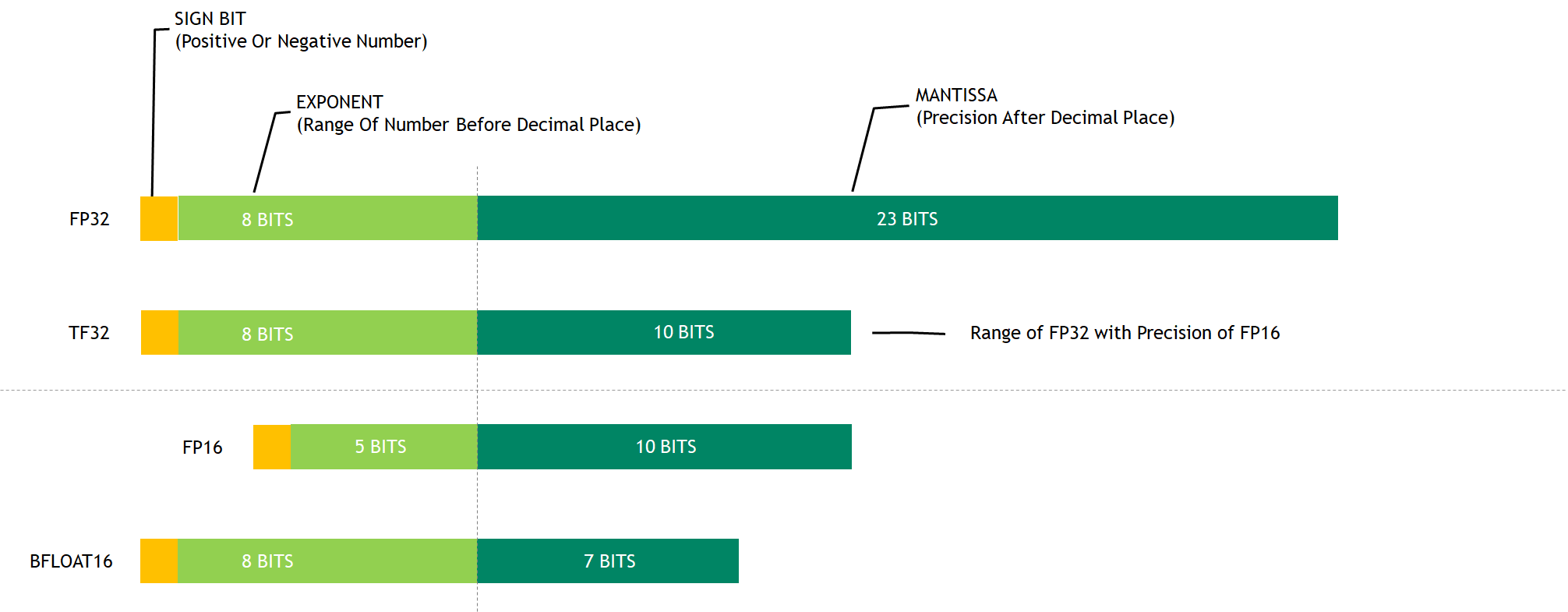
As mentioned earlier, using FP16 is relatively simple.

When using the API, you can set it in the config with config->setFlag(nvinfer1::BuilderFlag::kFP16); (C++) or builder_config.set_flag(trt.BuilderFlag.FP16) (Python). When converting ONNX models using trtexec, you can add the -fp16 flag.

4.6.2 Using INT8 in TensorRT

In INT8 quantization, a key step is determining the appropriate threshold (scale), which dictates how floating-point activations are mapped to 8-bit integers.

Initially, by statistically analyzing the activations of each layer in the model, it is observed that most activation values are concentrated within a lower range, with very few large activation values. This suggests that using saturation quantization (mapping the maximum activation value to 127) might not be optimal, as it wastes quantization range on a small number of large activation values.

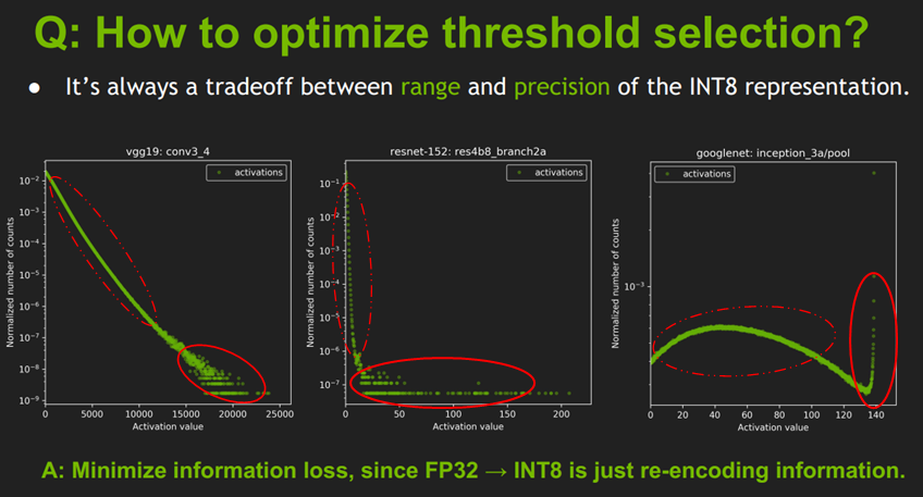
To more effectively utilize the quantization range, TensorRT adopts a dynamic threshold determination method. The specific approach is:

1. Divide the activation values of each layer's feature map into 2048 bins, with each bin representing a range of activation values.
2. Starting from the 127th bin, attempt to use the midpoint of each bin as a threshold and compute the corresponding quantization results.
3. For each attempted threshold, map activation values below that threshold to integers between 0-127, and map activation values above the threshold to 127.
4. Generate a 128-dimensional distribution vector representing the number of elements for each quantized value.
5. Evaluate the reasonableness of each threshold by calculating the similarity (using KL divergence) between the original distribution (2048 bins) and the quantized distribution (128-dimensional vector).
6. Select the threshold that minimizes the KL divergence as the final scale.

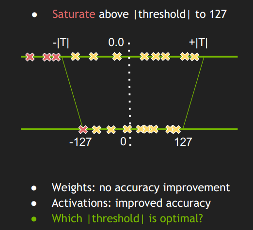
The core of this method is dynamically adjusting the threshold so that the quantized distribution closely matches the original distribution, thereby minimizing the information loss caused by quantization. This allows for reducing the computational and storage demands of the model while maintaining its performance. This method requires a calibration dataset to determine the quantization parameters.

Example Using BERT

Using BERT as an example, we'll explain how to perform INT8 quantization. Unlike FP16, INT8 requires preparing a calibration dataset and defining a custom calibrator class that inherits from trt.IInt8EntropyCalibrator.

Preparing the Dataset

The method for obtaining BERT input is similar to the API used earlier, where the input text is converted into a format suitable for the model. Specifically, it uses a tokenizer to encode the text and generate the required input tensors for the model.

def text2inputs(tokenizer, text):
    encoded_input = tokenizer.encode_plus(text, return_tensors = "pt")

    input_ids = encoded_input['input_ids'].int().detach().numpy()
    token_type_ids = encoded_input['token_type_ids'].int().detach().numpy()
    # position_ids = Torch.arange(0, encoded_input['input_ids'].shape[1]).int().view(1, -1).numpy()
    seq_len = encoded_input['input_ids'].shape[1]
    position_ids = np.arange(seq_len, dtype = np.int32).reshape(1, -1)
    input_list = [input_ids, token_type_ids, position_ids]

    return input_list

Implementing a Calibrator Class

The BERTCalibrator class is used for performing INT8 quantization calibration of a BERT model in TensorRT and inherits from trt.IInt8EntropyCalibrator. It reads the text data, converts it into a model input format, and provides these inputs during calibration. The class also implements the functionality to read and write calibration caches, allowing calibration data to be reused across multiple runs.

class BERTCalibrator(trt.IInt8LegacyCalibrator):
    def __init__(self, data_txt, BERT_path, cache_file, batch_size, max_seq_length, num_inputs):
        trt.IInt8LegacyCalibrator.__init__(self)

        tokenizer = BERTTokenizer.from_pretrained(BERT_path)
        self.tokenizer = BERTTokenizer.from_pretrained(BERT_path)

        self.input_ids_list = []
        self.token_type_ids_list = []
        self.position_ids_list = []
        with open(data_txt, "r") as f:
            lines = f.readlines()
            for i in range(0, num_inputs):
                inputs = text2inputs(tokenizer, lines[i])
                self.input_ids_list.append(inputs[0])
                self.token_type_ids_list.append(inputs[1])
                self.position_ids_list.append(inputs[2])
                if i % 10 == 0:
                    print("text2inputs:" + lines[i])

        self.cache_file = cache_file
        # Every time get_batch is called, the next batch of size batch_size will be copied to the device and returned.
        self.max_seq_length = max_seq_length
        self.batch_size = batch_size
        self.current_index = 0
        if num_inputs > len(self.input_ids_list):
            self.num_inputs = len(self.input_ids_list)
        else:
            self.num_inputs = num_inputs
        self.doc_stride = 128
        self.max_query_length = 64

        # Allocate enough memory for a whole batch.
        self.device_inputs = [cuda.mem_alloc(self.max_seq_length * trt.int32.itemsize * self.batch_size) for binding in range(3)]

    def free(self):
        for dinput in self.device_inputs:
            dinput.free()

    def get_batch_size(self):
        return self.batch_size
    def get_batch(self, names):
        if self.current_index + self.batch_size > self.num_inputs:
            print("Calibrating index {:} batch size {:} exceed max input limit {:} sentences".format(self.current_index, self.batch_size, self.num_inputs))
            return None

        current_batch = int(self.current_index / self.batch_size)
        if current_batch % 10 == 0:
            print("Calibrating batch {:}, containing {:} sentences".format(current_batch, self.batch_size))

        input_ids = self.input_ids_list[self.current_index]
        token_type_ids = self.token_type_ids_list[self.current_index]
        position_ids = self.position_ids_list[self.current_index]

        seq_len = input_ids.shape[1]
        if seq_len > self.max_seq_length:
            print(seq_len)
            print(input_ids.shape)
            input_ids = input_ids[:, :self.max_seq_length]
            token_type_ids = token_type_ids[:, :self.max_seq_length]
            position_ids = position_ids[:, :self.max_seq_length]
            print(input_ids.shape)

        cuda.memcpy_htod(self.device_inputs[0], input_ids.ravel())
        cuda.memcpy_htod(self.device_inputs[1], token_type_ids.ravel())
        cuda.memcpy_htod(self.device_inputs[2], position_ids.ravel())

        self.current_index += self.batch_size
        return self.device_inputs

    def read_calibration_cache(self):
        # If there is a cache, use it instead of calibrating again. Otherwise, implicitly return None.
        if os.path.exists(self.cache_file):
            with open(self.cache_file, "rb") as f:
                return f.read()

    def write_calibration_cache(self, cache):
        with open(self.cache_file, "wb") as f:
            f.write(cache)
            f.flush()
            os.fsync(f)

    def get_quantile(self):
        return 0.9999

    def get_regression_cutoff(self):
        return 1.0

    def read_histogram_cache(self, length):
        return None

    def write_histogram_cache(self, ptr, length):
        return None

During the initialization of the BERTCalibrator class, the following steps are performed:

• Calling the Parent Class Constructor: The constructor of the parent class, trt.IInt8LegacyCalibrator, is called using trt.IInt8LegacyCalibrator.init(self).
• Initializing the Tokenizer: The BERTTokenizer is initialized from a pretrained BERT model path to handle the tokenization of input text.
• Reading and Processing Data: The text data is read from a file and then converted into the BERT model's input format (input_ids, token_type_ids, position_ids) using the text2inputs function.
• Setting Calibration Parameters: Essential calibration parameters such as the cache file path, batch size, and maximum sequence length are set.
• Allocating GPU Memory: Sufficient GPU memory is allocated to store the data for the entire batch.

Key Functions to Implement and Pay Attention To:

• get_batch_size(): This function returns the batch size for the calibration process.
• get_batch: This method retrieves the next batch of input data based on the current index and copies it to GPU memory. If the current index plus the batch size exceeds the total number of input data, it returns None.
• read_calibration_cache: This method checks if a calibration cache file exists. If it does, the cache is read and used for calibration.
• write_calibration_cache: This method writes the calibration cache to a file, allowing it to be reused in future runs.
• get_quantile 和 get_regression_cutoff: These methods return specific parameters required for quantization, such as the quantile for quantile-based calibration or the regression cutoff.
• read_histogram_cache 和 write_histogram_cache: These methods are used to read from and write to the histogram cache, which helps in preserving the distribution of activation values for more accurate quantization.

5. References

https://huggingface.co/blog/BERT-101

https://arxiv.org/pdf/1810.04805

https://jalammar.github.io/a-visual-guide-to-using-BERT-for-the-first-time/

https://wmathor.com/index.php/archives/1438/

https://luweikxy.gitbook.io/machine-learning-notes/self-attention-and-transformer#encoder-mo-kuai

https://armanasq.github.io/nlp/self-attention/

https://adaning.github.io/posts/52648.html#toc-heading-1

https://github.com/NVIDIA/FasterTransformer/blob/main/docs/BERT_guide.md#run-fastertransformer-BERT-on-c

https://github.com/NVIDIA/TensorRT/tree/release/10.0/demo/BERT

https://arxiv.org/pdf/2210.03052

https://arleyzhang.github.io/articles/923e2c40/