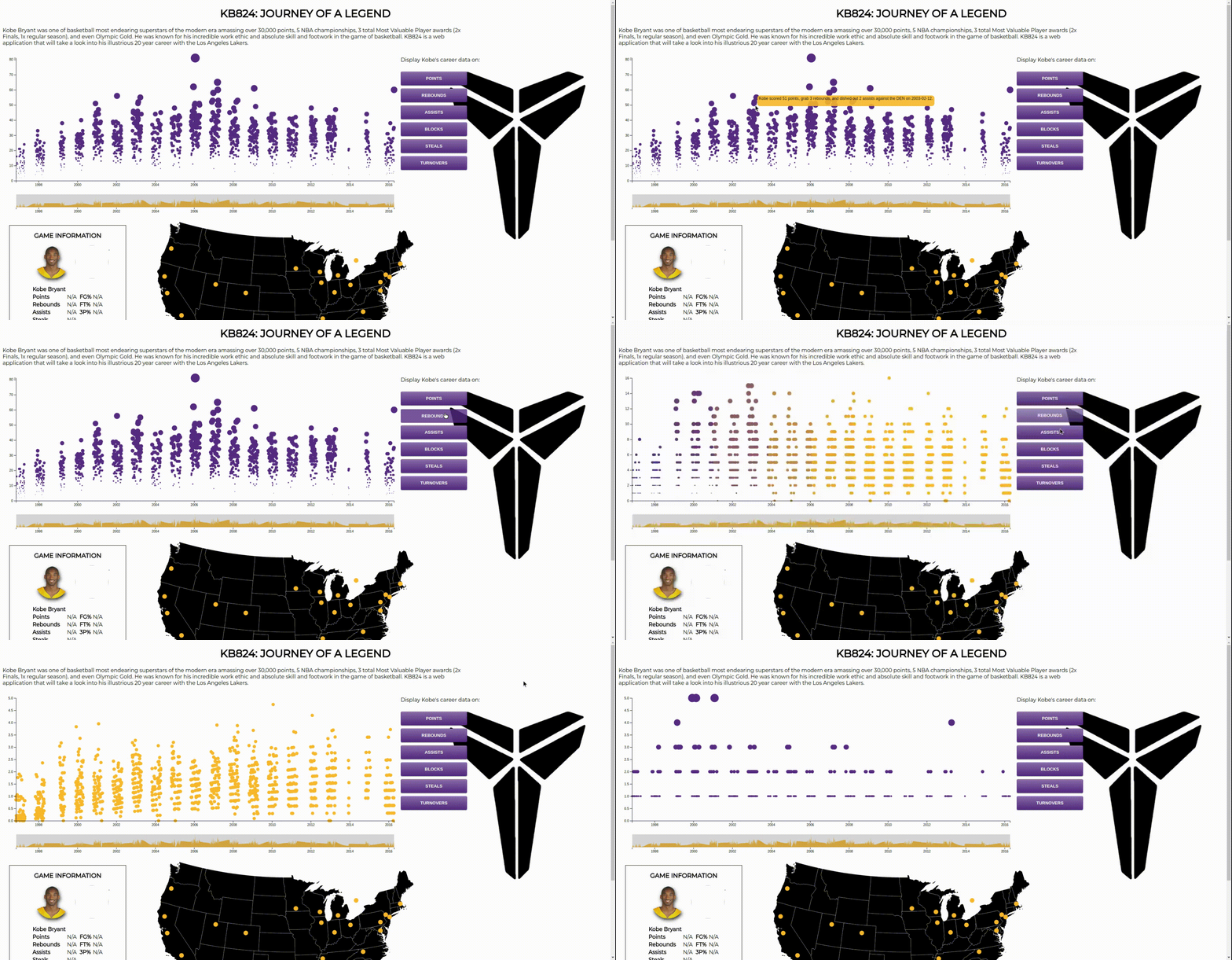
Kobe Bryant was one of basketball most endearing superstars of the modern era amassing over 30,000 points, 5 NBA championships, and 3 total Most Valuable Player awards (2x Finals, 1x regular season). He was known for his incredible work ethic and absolute dedication to the game and whose influence is beginning to mature in the superstars of today.
KB824 is a web application that will take a look into his illustrious 20 year career with the Los Angeles Lakers using vanilla JavaScript and a JavaScript library known as d3 to bring the data to life.
UPDATE: On January 26, 2020, a world lost an icon. Kobe was doing what he does best, being a father, and was on his way taking his beautiful and talented daugther Gianna to a youth game. On the way there, reduced visibility caused the heliocopter to crash killing all 9 aboard. While my heart is still heavy, I know his memories and teachings will still endure the test of time. Thank you Kobe for everything you did. Much love. Mamba out 🎤
Technologies Used
You can use a small HTTP server to fire up this webpage. For this example, we can use python3 to run a simple local HTTP server. Run the following command once python3 is installed in the directory you wish to run the server on
python3 -m http.serverThe dataset for the games played was obtained by webscraping from basketball reference sites. This was done using SuperAgent, a small progressive client-side HTTP request library and Cheerio, a library which parses markups and provides an API for traversing/manipulating the resulting DOM data structure. The API call is as follow and was very short itself. Meaningful cleaning of the data had to be performed after extraction of the data ad if I had to do it again, I would look to see if I could extract the data more cleanly.
superagent
  .get(url)
  .query()
  .end(function(err,response){
    if (err) {
      res.json({
        confirmation: "fail",
        message: err
      });
      return;
    }

    $ = cheerio.load(response.text);
    // var gameTable = $('#pgl_basic.1');
    // console.log(gameTable);
    $(`pgl_basic.1`).each((i,element)=>{
      console.log(element);
      console.log(i);
    });
    res.send(response.text);
});In all, over 1400 different nodes (games) were harvested and cleaned. The data was formatted into a comma separated value (CSV), a format parsable to D3. A snippet of each node can be seen below:
Rk,G,Date,Age,Tm,,Opp,,GS,MP,FG,FGA,FG%,3P,3PA,3P%,FT,FTA,FT%,ORB,DRB,TRB,AST,STL,BLK,TOV,PF,PTS,GmSc
1,1,1996-11-03,18-072,LAL,,MIN,W (+6),0,6:00,0,1,.000,0,0,,0,0,,0,1,1,0,0,1,1,1,0,-1.1
Some feature of this chart is the ability to dynamically change the value of the scatterplot node from an event listen handler install on a button. This causes the data to display the new stat triggering a transition for each of the nodes as well as transforming the axis as necessary.
Each stat is dynamically rendered in real time by having D3 dynamically manipulate the DOM using special jQuery-like selector methods like select. This triggers special event handlers that manipulating the current data on the DOM, changing it value. Each node is then "animated" using transition method to create a visually appealing rellocation of resources. The x and y-axes also scale accordingly when invoked with Javascript method call.
d3.select(".pts") //Points
    .on("click", function() {
        y.domain([0, d3.max(data, function(d) {
          return d.PTS; })]);

        // Update circles
        svg.selectAll("circle")
            .data(data)  // Update with new data
            .transition()  // Transition from old to new
            .duration(1000)  // Length of animation
            .on("start", function() {  // Start animation
                d3.select(this)  // 'this' means the current element
                    .attr("fill", "#FDB927")
                    // .attr("fill", "red")  // Change color
                    .attr("r", 5);  // Change size
            })
            .delay(function(d, i) {
                return i / data.length * 500;  // Dynamic delay (i.e. each item delays a little longer)
            })
            .attr("cx", function(d) {
                return x(d.date);  // Circle's X
            })
            .attr("cy", function(d) {
                return y(d.PTS);  // Circle's Y
            })
            .on("end", function() {  // End animation
                d3.select(this)  // 'this' means the current element
                    .transition()
                    .duration(500)
                    .attr("fill", "#552583")
                    .attr("r", (d)=>{return (d.PTS/6)});  // Change radius
            });

            // Update X Axis
            svg.select(".axis--x")
                .transition()
                .duration(1000)
                .call(xAxis);

            // Update Y Axis
            svg.select(".axis--y")
                .transition()
                .duration(100)
                .call(yAxis);
});Another highlight of this application is the interactive US Map. This map was created by passing in latitudinal and longitudinal coordinates into a function that will spit out the proper pixel x pixel 2D coordinates. This is then spit into a variable that maps the path given by these coordinates to create a US Map. Some more features are planned!
let projection = d3.geoAlbersUsa();
let path = d3.geoPath()
.projection(projection);
The actual conquest routes was generating on the fly using handrolled algorithms that calculate the data when it was being parsed in the scatterplot to output useful game information like PPG and GP. Using this information, I perform a simple sort to obtain the cities with the lowest scoring average to the highest.
//Kobe points against every arena
let sortedArenaPoints = [];
for (let team in teamAvg) {
    sortedArenaPoints.push([team, teamAvg[team]]);
}

sortedArenaPoints.sort(function(a, b) {
    return a[1] - b[1];
});
This data is dynamically render with D3 line that are staggered creating a unique visually stimulation of being on a roadtrip.
let links = [];
for(let i=0; i < data.length-1; i++){
    links.push({
        coordinates: [
            [ data[i].lon, data[i].lat ],
            [ data[i+1].lon, data[i+1].lat ]
        ]
    });
}

// Standard enter / update

for (let i = 0; i < links.length; i++) {
  svg2.selectAll(`line${i}`)
  .data(links)
  .enter()
  .append(`line`)
  .attr("x1", projection(links[i].coordinates[0])[0])
  .attr("y1", projection(links[i].coordinates[0])[1])
  .attr("x2", projection(links[i].coordinates[0])[0])
  .attr("y2", projection(links[i].coordinates[0])[1])
  .transition()
  .duration(2000)
  .delay(2000*i)
  .attr("x2", projection(links[i].coordinates[1])[0])
  .attr("y2", projection(links[i].coordinates[1])[1])
  .style("stroke","#552583")
  .style("stroke-width","2");

}

