-
Notifications
You must be signed in to change notification settings - Fork 60
Dam break VOF
VOF simulation of dam break: A liquid is fixed at an initial rectangular domain. At t = 0 s, the dam is removed and the liquid is released into the total simulation domain. The corresponding parameter file is gls_VOF_dam-break_Martin_and_Moyce.prm.
The following schematic describes the simulation.

slip and an external gravity field of -1 is applied in the y direction.
📣 This example simulates the dam break experiments of Martin and Moyce (1952). The link to this article: https://royalsocietypublishing.org/doi/abs/10.1098/rsta.1952.0006
Time integration is defined by a 1st order backward differentiation (bdf1), for a 4.1 seconds simulation (time end) with an initial time step of 0.01 seconds.
💡 This example uses an adaptative time-stepping method in which the time-steps are modified during the simulation to keep the max cfl constant.
# --------------------------------------------------
# Simulation Control
#---------------------------------------------------
subsection simulation control
  set method                  		= bdf1
  set time end                		= 4.1
  set time step               		= 0.01
  set adapt 		      		= true
  set max cfl		      		= 0.5
  set stop tolerance          		= 1e-5
  set adaptative time step scaling 	= 1.1
  set number mesh adapt       		= 0
  set output name             		= dam-break_VOF
  set output frequency        		= 20
  set output path                  	= ./Output/
  set subdivision             		= 1
end
The multiphysics subsection enables to turn on (true) and off (false) the physics of interest. Here VOF and interface sharpening are chosen.
❗ If the interface sharpening is not selected, the interface between phases will become blurry (due to diffusion). The following section defines the interface sharpening parameters.
#---------------------------------------------------
# Multiphysics
#---------------------------------------------------
subsection multiphysics
  set VOF = true
  set interface sharpening = true
end
In the interface sharpening subsection, the parameters required for sharpening the interface are defined. The current interface sharpening method consists of two steps. In the following, these steps and the implemented equations are explained:
1️⃣ phase fraction limiter (limits the phase fractions between 0 and 1 before interface sharpening:
2️⃣ interface sharpener:
where ,
c, and
denote phase fraction before interface sharpening, updated phase fraction after interface sharpening,
sharpening threshold, and interface sharpness, respectively. This interface sharpening method was proposed by Aliabadi and Tezduyar (2000): https://www.sciencedirect.com/science/article/pii/S0045782500002000
sharpening frequency is an integer parameter that defines the frequency of interface sharpening; sharpening threshold defines a phase fraction threshold for interface sharpening (generally 0.5); and interface sharpness is a model parameter which is generally in the range of (1-2].
#---------------------------------------------------
# Interphase sharpening
#---------------------------------------------------
subsection interface sharpening
  set sharpening threshold              = 0.5
  set interface sharpness               = 2
  set sharpening frequency      	= 10
end
In the initial condition, the initial velocity and initial position of the liquid phase are defined. The liquid phase is initially surrounded by a rectangle of length = 3.5 and height = 7.
#---------------------------------------------------
# Initial condition
#---------------------------------------------------
subsection initial conditions
    set type = nodal
    subsection uvwp
            set Function expression = 0; 0; 0
    end
    subsection VOF
            set Function expression = if (x<3.5 & y<7 , 1, 0)
    end
end
The source term subsection defines the gravitational acceleration:
#---------------------------------------------------
# Source term
#---------------------------------------------------
subsection source term
    set enable = true
    subsection xyz
        set Function expression = 0;-1.0; 0
    end
end
Two fluids are present in this simulation, hence in the physical properties subsection, their physical properties should be defined:
#---------------------------------------------------
# Physical Properties
#---------------------------------------------------
subsection physical properties
  set number of fluids     = 2
  subsection fluid 0
    set density              = 0.02
    set kinematic viscosity  = 0.1
  end
    subsection fluid 1
    set density              = 0.9982
    set kinematic viscosity  = 0.01
  end
end
In the mesh adaptation subsection, adaptive mesh refinement is defined for velocity. min refinement level and max refinement level are 4 and 5, respectively.
#---------------------------------------------------
# Mesh Adaptation
#---------------------------------------------------
subsection mesh adaptation
  set type                    = kelly
  set variable                = velocity
  set fraction type           = fraction
  set max refinement level    = 5
  set min refinement level    = 4
  set frequency               = 5
  set fraction refinement     = 0.2
  set fraction coarsening     = 0.01
end
✔️ The gls_navier_stokes_2d solver should be used for this simulation.
The following image shows the screenshots of the simulation at 0, 1.1, 3, and 4 s.

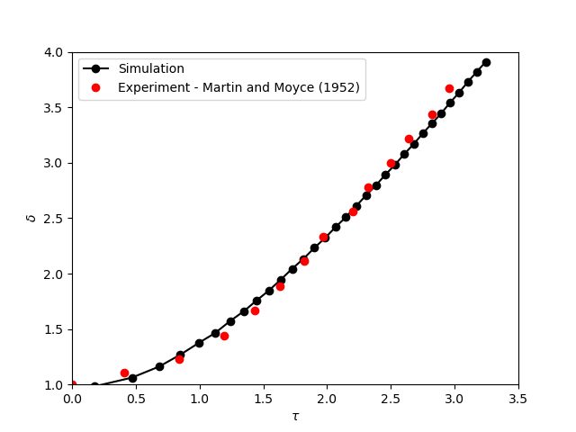
A python post-processing code (gls_VOF_dam-break_Martin_and_Moyce.py) is added to the example folder for post-processing the results. python3 ./Dambreak_2d_lethe.py ./Output executes this post-processing code, where ./Output is the directory that contains the simulation results. In post-processing, the maximum dimensionless lateral position of the liquid phase is tracked through time and compared with the experiments of Martin and Moyce (1952). The following figure shows the result of the post-processing:

As mentioned previously, this simulation uses adaptive mesh refinement. The following image shows the mesh and the position of the interface at 4 s. The mesh refinement detects and refines the meshes on the interface.
