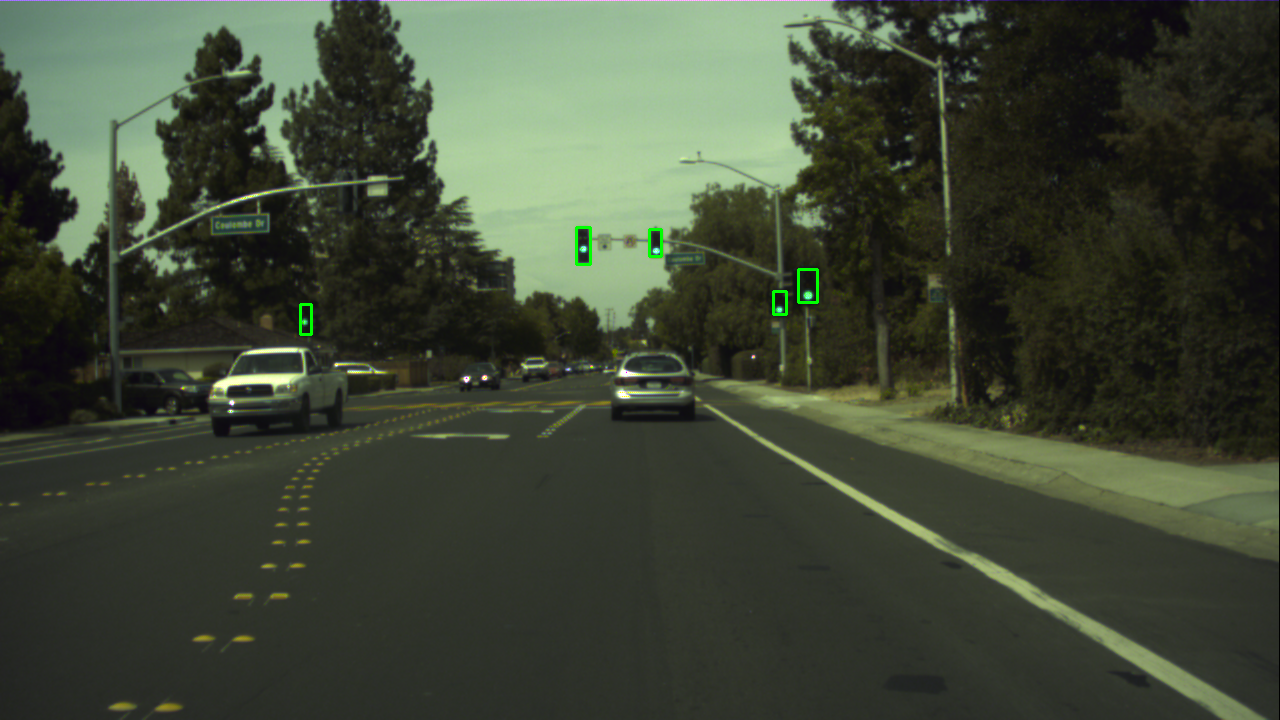
Using the Bosch dataset, this is a machine learning project that will be able to identify whether a traffic light in an image is red, green, or, yellow. The Bosch dataset has testing and training data on their website, but I decided to switch them because the training data had a couple of errors in the annotations. In addition, I wanted the training to have more images than test. My training dataset had 8334 images and my testing dataset had 5093 images, all with a resolution of 1280 x 720 pixels.
- Demo Video
- Usage
- Data Visulization
- Convolutional Neural Network
- Training Process
- Evaluation
- Further Discussion
- Contact
- References
This video shows the end result of my Convolutional Neural Network's classification of the annotated traffic lights. Because it is not 100% accurate, the colors might be off in some frames.
preprocessing.py
Extrapolates data from the YAML file, filters out the occluded and off labels, crops images and sorts them into folders, draws the bounding boxes.
visualization.py
Prints out statistics about the dataset, including drawing graphs about the distribution, heights, widths, and sizes.
train.py
The body of the CNN, normalizes all images to be 32 x 32 pixels, iterates through 10 epochs, printing out the loss for both train and validation, saves the model locally.
eval.py
Tests for accuracy in each of the datasets, prints out accuracy for each label as well, prints confusion matrix.
Examples of training images, with the traffic lights outlined in the color they are annotated in.
Many of the images were either occluded, off, or too small. For some, even a human eye would not be able to detect which color the light was.
The test dataset has a similar distribution. There are a lot fewer yellow data than green data, which contributes to the lower accuracy for data with ground truth yellow.
Convolutional neural networks (CNN) are used in machine learning, specifially when dealing with images, in order to build models that can label data. They are comprised of layers of "neurons" that are very similar to brain neurons- they take information from the previous layer and processes it, giving an output of the modified information. In convolutional neural networks, they give the input tensor a weight and bias using the formula y = wx + b. This is also known as a convolution layer. Other layers can have activation functions, which help the neuron decide if it will fire or not. Many activation functions are used today, but the most popular one and the one I used is what is known as ReLU, aka Rectified Linear Unit. Pooling layers reduce the number of parameters in the network and make the information easier to process. The last couple of layers are usually fully connected layers, where they are connected to all the activations from previous layers.
The input for this CNN is an image and the output is a matrix of probabilities, size three. The first number is green, the second is red, and the third is yellow. The greater the number, the more likely the model thinks it is.
This is a graph of what my CNN looks like:
To train, I used a decaying learning rate, starting from 0.001 and decaying by 1/5 every time the change in loss is less than 5 times the learning rate. Trial and error taught me that 0.001 was the optimal learning rate to begin with because 0.01 would overshoot and 0.0001 would be too slow to converge.
In order to see if my model was overfitting the data, I split the training data into train and validation, in an 8:2 ratio. Here is the plot of training loss versus validation loss:
As you can see, the validation loss is always below the training loss, suggesting that there is no overfitting. Note that the y-axis is log scale.
After training the model, I evaluated it on the dataset. Accuracy for the training data was 99% (4897/4898), validation was 100% (1225/1225), and test was 91% (2705/2941). Because it is a lot higher than 33%, I know that it was not randomly guessing and was actually able to identify most of the cases.
Inside the test data, the model predicted 97% (1682/1730) of green, 92% (964/1042) of red, and 34% (59/169) of yellow. As expected, yellow was the most inaccurate, due to the very few training data of yellow.
| Test | Validation | Train |
|---|---|---|
| 99% | 100% | 91% |
| 4897/4898 | 1225/1225 | 2705/2940 |
| Green | Red | Yellow |
|---|---|---|
| 97% | 92% | 34% |
| 1682/1730 | 964/1042 | 59/169 |
| Classifier Results \ Truth Data | Red | Green | Yellow | Total | Precision |
|---|---|---|---|---|---|
| Red | 1682 | 61 | 73 | 1816 | 92.621% |
| Green | 26 | 964 | 37 | 1027 | 93.866% |
| Yellow | 22 | 17 | 59 | 98 | 60.204% |
| Total | 1730 | 1042 | 169 | 2941 | |
| Recall | 97.255% | 92.514% | 34.911% |
This entire project used annotations from the Bosch dataset. Later, this can expand to image segmentation so that it can identify where the traffic lights are from any image, in addition to classifying them. Also, this was a simplified version of the problem, with all the arrow cases removed and all the traffic lights smaller than 5 pixels wide and 10 pixels long removed. If this can expand further, we can implement this piece of code into a physical device than can be attached to a windshield, identifying traffic lights in real time.
If you have any questions, feel free to contact me at [email protected]!


