-
Notifications
You must be signed in to change notification settings - Fork 332
YModel practice:Use historical data for business forecasting
Before getting started with YModel, the first thing we should do is to make the objective clear, that is to say, we should know what we want to predict.
For example, when granting a loan, the bank wants to predict the possibility of borrower default, so as to determine whether to provide a loan and confirm the loan interest rate.
When setting premiums, the insurance company wants to predict the risk of customer claims, so as to formulate more flexible premium policies.
In business marketing, the company wants to predict which customers will purchase which products and thus carry out sales activities more precisely, and so on.
As long as we have enough historical data, all of these tasks can be accomplished.
Let’s take loan default prediction as an example. We can collect recent loan data as historical data. For example, if we want to predict customer default in July, the data from January to June, or the data for the past year, or the data for the past three months, etc., can be collected to build a model. Which data to collect depends on the business characteristics.
The collected historical data need to be arranged into a table like the one below, which is commonly known as a wide table.
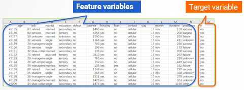
The wide table should contain feature variables and target variable.
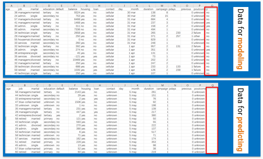
The target variable is the objective to be predicted, such as the variable y in the figure. This variable represents the default situation of each loan, and it has two values: yes and no, where ‘yes’ indicates default, and ‘no’ indicates no default.
The feature variables refer to the information that may be related to the prediction objective.
For example, in this example, the feature variables include the information of borrowers, such as income level, debt situation, loan amount, term, interest rate, job, housing condition.
This type of problem where the target variable has only two values, yes and no, is called the binary classification problem, which is a very common prediction type. For example, predicting whether a customer will buy a certain product, whether a platform will churn users, whether an email is spam, etc., all fall under binary classification problem.
In addition, YModel can also solve regression and multi-classification problems.
The regression problem refers to a problem where the target variable is a numerical value, such as predicting the sales volume or selling price of a product.
The multi-classification problem generally refers to predicting which category something belongs to, such as predicting whether a product’s grade is excellent, good, qualified or poor.
Having arranged data into a wide table, save it in Excel format, or in csv or txt format, any of which is acceptable.
Once the wide table is ready, we can use it for modeling.
Click on the ‘New model’ button, select the prepared wide table, and import it in YModel.
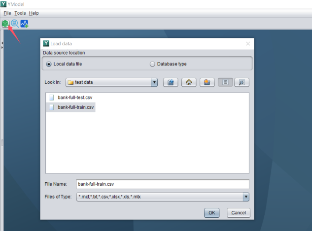
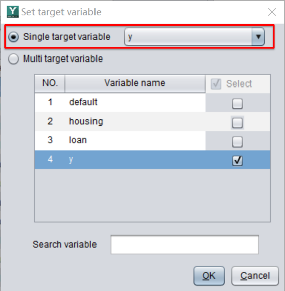
After importing the wide table, YModel will prompt you to configure the target variable.
For example, the target variable in this dataset is y, which indicates whether the customer will default.
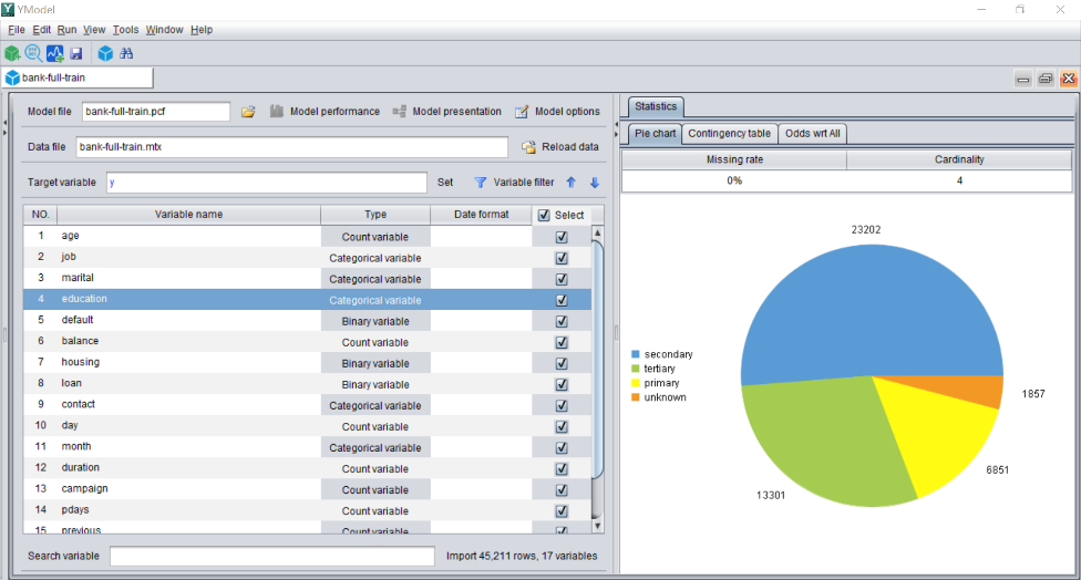
YModel will also automatically identify the data types of these feature variables and draw analysis charts.
For example, the variable ‘education’ in this example represents the educational level the borrowers. YModel identified it as a categorical variable with a missing rate of 0. This variable has 4 categories, among which the category ‘secondary’ has the largest number of values, corresponding to the blue part in the pie chart, and accounting for approximately 51%.
Now just click on the ‘Modeling’ button on the toolbar, the entire data preprocessing and modeling process will proceed automatically and does not require manual operation.

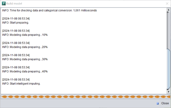
A progress bar will be displayed during modeling. As shown in the figure below, it indicates the data preprocessing has advanced to 40%.
It will take about a few minutes to several tens of minutes to build a model, sometimes even shorter, depending on the amount of data.
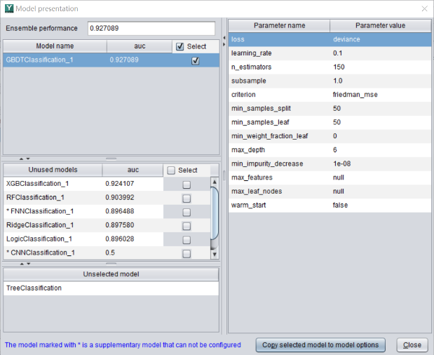
After the model is built, you can see the model’s algorithms and corresponding parameters. and at the same time, YModel will output a model file with a suffix ‘.pcf’, which is used for prediction.
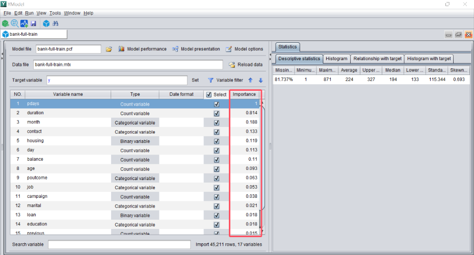
Once the modeling process is finished, an interface that displays the importance of each variable will appear.
The larger the importance, the greater the variable affects the prediction objective.
This function can help us conduct some business analysis. For example, the variable ‘pdays’ in the dataset has a greater impact on customer default.
After a model is built, clicking on ‘Model performance’ can view the model’s performance for evaluation.
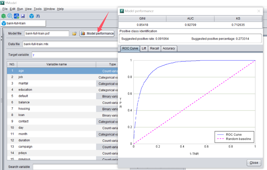
For example, we will often see an indicator called AUC, and its value range is (0.5-1). In principle, the higher the value the better the performance.
In this example, the model’s AUC is 0.927, which indicates it is a good model. Using this model for prediction will yield highly reliable results.
Once the model is evaluated as qualified, prediction can be made.
The data to be predicted should also be a wide table. In this table, the feature variables must be consistent with the those used for modeling, except that it does not contain the target variable.
For example, there are two tables in the following figure. The upper table is the data for modeling and contains the target variable y.
The lower table is the data to be predicted, and does not contain the target variable y. Apart from this, the names of the other variables are the same.
Open the prediction interface, import the pcf model file, and then import the data set to be predicted. At this time, prediction can be performed.
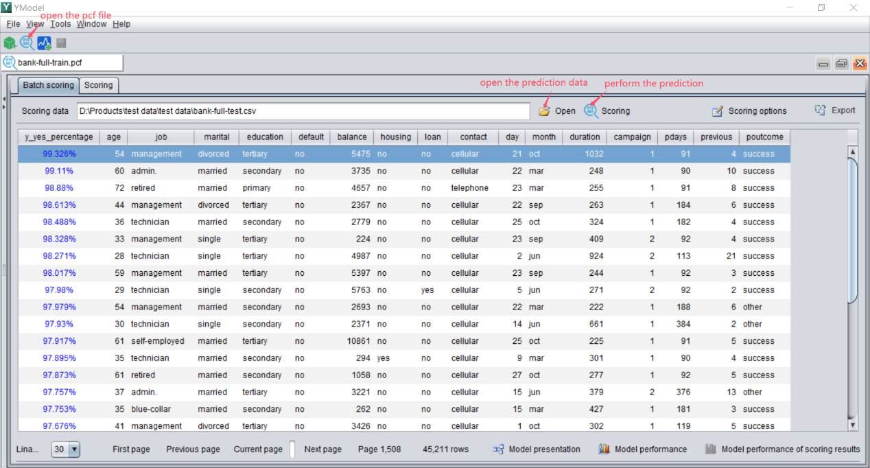
The interface presented in the figure above will be displayed following the completion of the prediction, and the leftmost column is the prediction results. In this example, the percentage represents the default probability of a customer. The higher the default probability, the higher the default risk.
Clicking on the variable name of this column can also sort the prediction results to screen out high-risk customers.
Finally, let’s summarize the process of using historical data for business forecasting.
1. Arrange data into wide table.
Arrange the historical data and the to-be-predicted data into a wide table respectively. The historical data must contain the target variable, while the to-be-predicted data should not contain the target variable.
2. Import data and build a model.
Import the historical data into YModel, build a model, and generate a model file with a suffix ‘.pcf’.
3. Use the model to make prediction.
Open the pcf model file, import the to-be-predicted data, and execute prediction. Then, you can determine which actions to take based on the prediction results such as default probability.
SPL Resource: SPL Official Website | SPL Blog | Download esProc SPL | SPL Source Code